A sneak peek at Bayesian Inference
So far on this blog, we have looked the mathematics behind distributions, most notably binomial, Poisson, and Gamma, with a little bit of exponential. These distributions are interesting in and of themselves, but their true beauty shines through when we analyze them under the light of Bayesian inference. In today’s post, we first develop an intuition for conditional probabilities to derive Bayes’ theorem. From there, we motivate the method of Bayesian inference as a means of understanding probability.
Conditional Probability
Suppose a man believes he may have been affected with a flu after days of fever and coughing. At the nearest hospital, he is offered to undergo a clinical examination that is known to have an accuracy of 90 percent, i.e. it will return positive results to positive cases 90 percent of the time. However, it is also known that the test produces false positives 50 percent of the time. In other words, a healthy, unaffected individual will test positive with a probability of 50 percent.
In cases like these, conditional probability is a great way to package and represent information. Conditional probability refers to a measure of the probability of an event occurring, given that another event has occurred. Mathematically, we can define the conditional probability of event \(A\) given \(B\) as follows:
\[P(A \mid B) = \frac{P(A \cap B)}{P(B)}\]This equation simple states that the conditional probability of \(A\) given \(B\) is the fraction of the marginal probability \(P(B)\) and the area of intersection between those two events, \(P(A \cap B)\). This is a highly intuitive restatement of the definition of conditional probability introduced above: given that event \(B\) has already occurred, conditional probability tells us the probability that event \(A\) occurs, which is then synonymous to that statement that \(A \cap B\) has occurred.
By the same token, we can also define the reverse conditional probability of \(B\) given \(A\) through symmetry and substitution. Notice that the numerator stays unchanged since the operation of intersection is commutative.
\[P(B \mid A) = \frac{P(A \cap B)}{P(A)}\]Now let’s develop an intuition for conditional probabilities by applying it to our example of clinical trials and the potentially affected patient. The purported accuracy of the clinical test is 90 percent, which we might express as follows, using the conditional probability notation:
\[P(\text{test +} \mid \text{sick}) = 0.9\]By the same token, we can also express the information on false positives as shown below. This conditional probability statement espouses that, given an individual who is not sick, the test returns a false positive 50 percent of the time.
\[P(\text{test +} \mid \text{¬sick}) = 0.5\]Conditional probability provides us with an interesting way to analyze given information. For instance, let \(R\) be the event that it rains tomorrow, and \(C\) be the event that it is cloudy at the present moment. Although we are no experts in climatology and weather forecast, common sense tells us that
\[P(R \mid C) > P(R)\]since with the additional piece of information that current weather conditions are cloudy, we are inclined to believe that it will likely rain tomorrow, or in the near future. Like this, conditional probability allows us to update our beliefs on uncertainty given new information, and we will see in the later sections that this is the core idea behind Bayesian inference.
Bayes’ Theorem
Let’s return back to the example of the potential patient with a flu. Shortly afterwards at the hospital, the the man was convinced by the doctor and decided to take the clinical test, the result of which was positive. We cannot assume that the man is sick, however, since the test has a rather high rate of false positives as we saw earlier. In this situation, the parameter that is of interest to us can be expressed as
\[P(\text{sick} \mid \text{test +})\]In other words, given a positive test result, what is the probability that the man is actually sick? However, we have no means as of yet to directly answer this question; the two pieces of information we have are that \(P(\text{test +} \mid \text{sick}) = 0.9\), and that \(P(\text{test +} \mid \text{¬sick}) = 0.5\). To calculate the value of \(P(\text{sick} \mid \text{test +})\), we need Bayes’s theorem to do its trick.
Let’s quickly derive Bayes’ theorem using the definition of conditional probabilities delineated earlier. Recall that
\[P(A \mid B) = \frac{P(A \cap B)}{P(B)} \tag{1}\] \[P(B \mid A) = \frac{P(A \cap B)}{P(A)} \tag{2}\]Multiply \(P(B)\) and \(P(A)\) on both sides of (1) and (2) respectively to obtain the following result:
\[P(A \mid B) P(B) = P(A \cap B)\] \[P(B \mid A) P(A) = P(A \cap B)\]Notice that the two equations describe the same quantity, namely \(P(A \cap B)\). We can use equivalence to put these two equations together in the following form.
\[P(A \mid B) P(B) = P(B \mid A) P(A) \tag{3}\]Equation (3) can be manipulated in the following manner to finally produce a simple form of Bayes’ theorem:
\[P(B \mid A) = \frac{P(A \mid B) P(B)}{P(A)} \tag{4}\]We can motivate a more intricate version this rule by modifying the denominator. Given that \(A\) and \(B\) are discrete events, we can break down \(A\) as a union of intersections between \(A\) and \(B_i\), where \(B_i\) represents subsets within event \(B\). In concrete form, we can rewrite this as
\[P(A) = \sum_{i = 1}^n P(A \cap B_i)\]Additionally, we can rewrite the conditional probability \(P(A \cap B_i)\) in terms of \(P(B_i)\) and \(P(A \mid B_i)\) according to the definition of conditional probability we observed earlier. Applying these alterations to (4) to rewrite \(P(A)\) produces equation (5):
\[P(B_k \mid A) = \frac{P(A \mid B_k) P(B_k)}{\sum_{i = 1}^n P(A \mid B_i) P(B_i)} \tag{5}\]This is the equation of Bayes’ theorem. In simple language, Bayes’ theorem tells us that the conditional probability of some subset \(B_k\) given \(A\) is equal to its relevant fraction within a weighted summation of the conditional probabilities \(A\) given \(B_i\). Although this equation may seem complicated at a glance, we can develop an intuition for this formula by reminding ourselves of the definition of conditional probabilities, as well as the fact that independent events can be expressed as a union of intersections.
At the end of the day, Bayes’ theorem provides a powerful tool through which we can calculate a conditional probability in terms of its reverse, i.e. calculate \(P(B \mid A)\) by utilizing \(P(A \mid B)\). Why is this important at all? Let’s return back to our example of the potential patient. Recall that the conditional probability of our interest was
\[P(\text{sick} \mid \text{test +})\]while the pieces of information we were provided were
\[P(\text{test +} \mid \text{sick}) = 0.9, P(\text{test +} \mid \text{¬sick}) = 0.5\]This is where Bayes’ theorem comes in handy.
\[P(\text{sick} \mid \text{test +}) = \frac{P(\text{test +} \mid \text{sick}) P(\text{sick})}{P(test +)} = \frac{P(\text{test +} \mid \text{sick}) P(\text{sick})}{P(\text{test +} \mid \text{sick}) P(\text{sick}) + P(\text{test +} \mid \text{¬sick}) P(\text{¬sick})}\]Notice that we have expressed \(P(\text{sick} \mid \text{test +})\) in terms of \(P(\text{test +} \mid \text{sick})\) and \(P(\text{test +} \mid \text{¬sick}) P(\text{¬sick})\). From a statistics point of view, all we have to do now is conduct a random survey of the population to see the percentage of the demographic infected with the flu. Let’s say that 15 percent of the population has been affected with this flu. Plugging in the relevant value yields
\[P(\text{sick} \mid \text{test +}) = \frac{0.9 \cdot 0.15}{0.9 \cdot 0.15 + 0.5 \cdot 0.85} \approx 0.241\]Using Bayes’ theorem, we are able to conclude that there is roughly a 24 percent chance that the man who tests positive on this examination is affected by the flu. That seems pretty low given the 90 percent accuracy of the test, doesn’t it? This ostensible discrepancy originates from the fact that the test has a substantial false positive of 50 percent, and also that the vast majority of the population is unaffected by the disease. This means that, if the entire population were to conduct this test, there would be more false positives than there would be true positives; hence the distortion in the value of the conditional probability.
But what if the man were to take the same test again? Intuition tells us that the more test he takes, the more confident we can be on whether the man is or is not affected by the disease. For instance, if the man repeats the exam once and receives a positive report, the conditional probability that he is sick given two consecutive positive test results should be higher than the 24 percent we calculated above. We can see this in practice by reapplying Bayes’ theorem with updated information, as shown below:
\[P(\text{sick} \mid \text{test +}) = \frac{P(\text{test +} \mid \text{sick}) P(\text{sick})}{P(\text{test +} \mid \text{sick}) P(\text{sick}) + P(\text{test +} \mid \text{¬sick}) P(\text{¬sick})} = \frac{0.9 \cdot 0.241}{0.9 \cdot 0.241 + 0.5 \cdot 0.759} \approx 0.364\]We see that the value of the conditional probability has indeed increased, lending credence to the idea that the man is sick. Like this, Like this, Bayes’ theorem is a powerful tool that can be used to calculate conditional probabilities and to update them continuously through repeated trials. From a Bayesian perspective, we begin with some expectation, or prior probability, that an event will occur. We then update this prior probability by computing conditional probabilities with new information obtained for each trial, the result of which yields a posterior probability. This posterior probability can then be used as a new prior probability for subsequent analysis. In this light, Bayesian statistics offers a new way to compute new information and update our beliefs about an event in probabilistic terms.
Bayesian Inference
Bayesian inference is nothing more than an extension of Bayes’ theorem. The biggest difference between the two is that Bayesian inference mainly deals with probability distributions instead of point probabilities. The case of the potential patient we analyzed above was a simple yet illuminating example, but it was limiting in that we assumed all parameters to be simple constants, such as \(0.9\) for test accuracy and \(0.5\) for false positive frequency. In reality, most statistical estimates exist as probability distributions since there are limitations to our ability to measure and survey data from the population. For example, a simple random sampling of the population might reveal that 15 percent of the sample population is affected with the flu, but this would most likely produce a normal distribution with mean centered around 0.15 instead of a point probability. From a Bayesian standpoint, we would then replace the point probability in our example above with an equation for the distribution, from which we can proceed with the Bayesian analysis of updating our prior with the posterior through repeated testing and computation.
Bayes’ theorem, specifically in the context of statistical inference, can be expressed as
\[f(\theta \mid D) = \frac{f(D \mid \theta) f(\theta)}{f(D)} \tag{6}\]where \(D\) stands for observed or measured data, \(\theta\) stands for parameters, and \(f\) stands for some probability distribution. In the language of Bayesian inference, \(f(\theta \mid D)\) is the posterior distribution for the parameter \(\theta\), \(f(D \mid \theta)\) is the likelihood function that expresses the likelihood of having parameter \(\theta\) given some observed data \(D\), \(f(\theta)\) is the prior distribution for the parameter \(\theta\), and \(f(D)\) is evidence, the marginal probability of seeing the data, which is determined by summing or integrating across all possible values of the parameter, weighted by how strongly we believe in those particular values of \(\theta\). Concretely,
\[f(D) = \int f(D \mid \theta) f(\theta) \, d\theta\]Notice that this is not so different from the expansion of the denominator we saw with Bayes’ theorem, specifically equation (5). The only difference here is that the integral takes continuous probability density functions into account, as opposed to discrete point probabilities we dealt with earlier.
If we temporarily disregard the constants that show up in (6), we can conveniently trim down the equation for Bayesian inference as follows:
\[\text{Posterior} \propto \text{Likelihood} \cdot \text{Prior}\]This idea is not totally alien to us—indeed, this is precisely the insight we gleaned from the example of the potential patient. This statement is also highly intuitive as well. The posterior probability would be some mix of our initial belief, expressed as a prior, and the data newly presented, the likelihood. Bayesian inference, then, can be understood as a procedure for incorporating prior beliefs with evidence in order to derive an updated posterior. What makes Bayesian inference such a powerful technique is that the derived posterior can themselves be used as a prior for subsequent inference conducted with new data.
To see Bayesian inference in action, let’s dive into the most classic, beaten-to-death yet nonetheless useful example in probability and statistics: the coin flip. This example was borrowed from the following post.
The Coin Flip
Assume that we have a coin whose fairness is unknown. To be fair, most coins are approximately fair (no pun intended) given the physics of metallurgy and center of mass, but for now let’s assume that we are ignorant of coin’s fairness, or the lack thereof. By employing Bayesian inference, we can update our beliefs on the fairness of the coin as we accumulate more data through repeated coin flips. For the purposes of this post, we will assume that each coin flip is independent of others, i.e. the coin flips are independent and identically distributed.
Let’s start by coming up with a model representation of the likelihood function, which we might recall is the probability of having a parameter value of \(\theta\) given some data \(D\). It is not difficult to see that the best distribution for the likelihood function given the setup of the problem is the binary distribution since each coin flip is a Bernoulli trial. Let \(X\) denote a random variable that represents the number of tails in \(n\) coin flips. For convenience purposes, we define 1 to be heads and 0 to be tails. Then, the conditional probability of obtaining \(k\) heads given a fairness parameter \(\theta\) can be expressed as
\[L(\theta \mid k)= \binom{n}{k} \theta^k (1 - \theta)^{n - k}\]We can perform a quick sanity check on this formula by observing that, when \(\theta = 0\), the probability of observing \(k\) heads diminishes to 0, unless \(k = 0\), in which case the probability becomes 1. This behavior is expected since \(\theta = 0\) represents a perfectly biased coin that always shows tails. By symmetry, the same logic applies to a hypothetical coin that always shows heads, and represents a fairness parameter of 1.
Now that we have derived a likelihood function, we move onto the next component necessary for Bayesian analysis: the prior. Determining a probability distribution for the prior is a bit more challenging than coming up with the likelihood function, but we do have certain clues as to what characteristics our prior should look possess.
First, the domain of the prior probability distribution should be contained within \([0, 1]\). This is because the range of the fairness parameter \(\theta\) is also defined within this range. This constraint immediately tells us that
\[\int_0^1 f(x) = 1\]where \(f(x)\) is represents the probability density function that represents the prior. Recall that some of the other functions we have looked at, namely binomial, Poisson, Gamma, or exponential are all defined within the unclosed interval \([- \infty, \infty]\), making it unsuitable for our purposes.
The Beta distribution nicely satisfies this criterion. The Beta distribution is somewhat similar to the Gamma distribution we analyzed earlier in that it is defined by two shape parameters, \(\alpha\) and \(\beta\). Concretely, the probability density function of the Beta distribution goes as follows:
\[f(x; \alpha, \beta) = \frac{\Gamma(\alpha + \beta)}{\Gamma(\alpha) \Gamma(\beta)} x^{\alpha - 1} (1 - x)^{\beta - 1}\]The coefficient, expressed in terms of a fraction of Gamma functions, provides a definition for the Beta function.
\[\frac{\Gamma(\alpha + \beta)}{\Gamma(\alpha) \Gamma(\beta)} = \frac{1}{B(\alpha, \beta)}\]The derivation of the Beta distribution and its apparent relationship with the Gamma function deserves an entirely separate post devoted specifically to the said topic. For the purpose of this post, an intuitive understanding of this distribution and function will suffice. A salient feature of the Beta distribution that is domain is contained within \([0 ,1]\). This means that, application-wise, the Beta distribution is most often used to model a distribution of probabilities, say the batting average of a baseball player as shown in this post. It is also worth noting that the Beta function, which serves as a coefficient in the equation for the Beta PDF, serves as a normalization constant to ensure that integrating the function over the domain \([0, 1]\) would yield 1 as per the definition of a PDF. To see this, one needs to prove
\[\int_0^1 x^{\alpha - 1} (1 - x)^{\beta - 1} \, dx = B(\alpha, \beta)\]This is left as an exercise for the keen reader. We will revisit this problem in a separate post.
Another reason why the Beta distribution is an excellent choice for our prior representation is that it is a conjugate prior to the binomial distribution. Simply put, this means that using the Beta distribution as our prior, combined with a binomial likelihood function, will produce a posterior that also follows a Beta distribution. This fact is crucial for Bayesian analysis. Recall that the beauty of Bayesian inference originates from repeated applicability: a posterior we obtain after a single round of calculation can be used as a prior to perform the next iteration of inference. In order to ensure the ease of this procedure, intuitively it is necessary for the prior and the posterior to take the same form of distribution. Conjugate priors streamline the Bayesian process of updating our priors with posteriors by ensuring that this condition is satisfied. In simple language, mathematicians have found that certain priors go well with certain likelihoods. For instance, a normal prior goes along with a normal likelihood; Gamma prior, Poisson likelihood; Gamma prior, normal likelihood, and so on. Our current combination, Beta prior and binomial likelihood, is also up on this list.
To develop some intuition, here is a graphical representation of the Beta function for different values of \(\alpha\) and \(\beta\).
import numpy as np
import matplotlib.pyplot as plt
import seaborn as sns
from scipy.stats import beta

plt.style.use("seaborn")
x = np.linspace(0, 1, 100)
params = [(0.5, 0.5), (1, 1), (5, 3), (2, 5), (10, 10)]
colors = ["c-", "m-", "g-", "y", "r-"]

for p, c in zip(params, colors):
	y = beta.pdf(x, p[0], p[1])
	plt.plot(x, y, c, label="$\\alpha=%s$, $\\beta=%s$" % p)

plt.grid(True)
plt.xlabel("$\\theta$")
plt.ylabel("Density")
plt.title('Beta Distribution')
plt.legend()
plt.show()
This code block produces the following diagram.
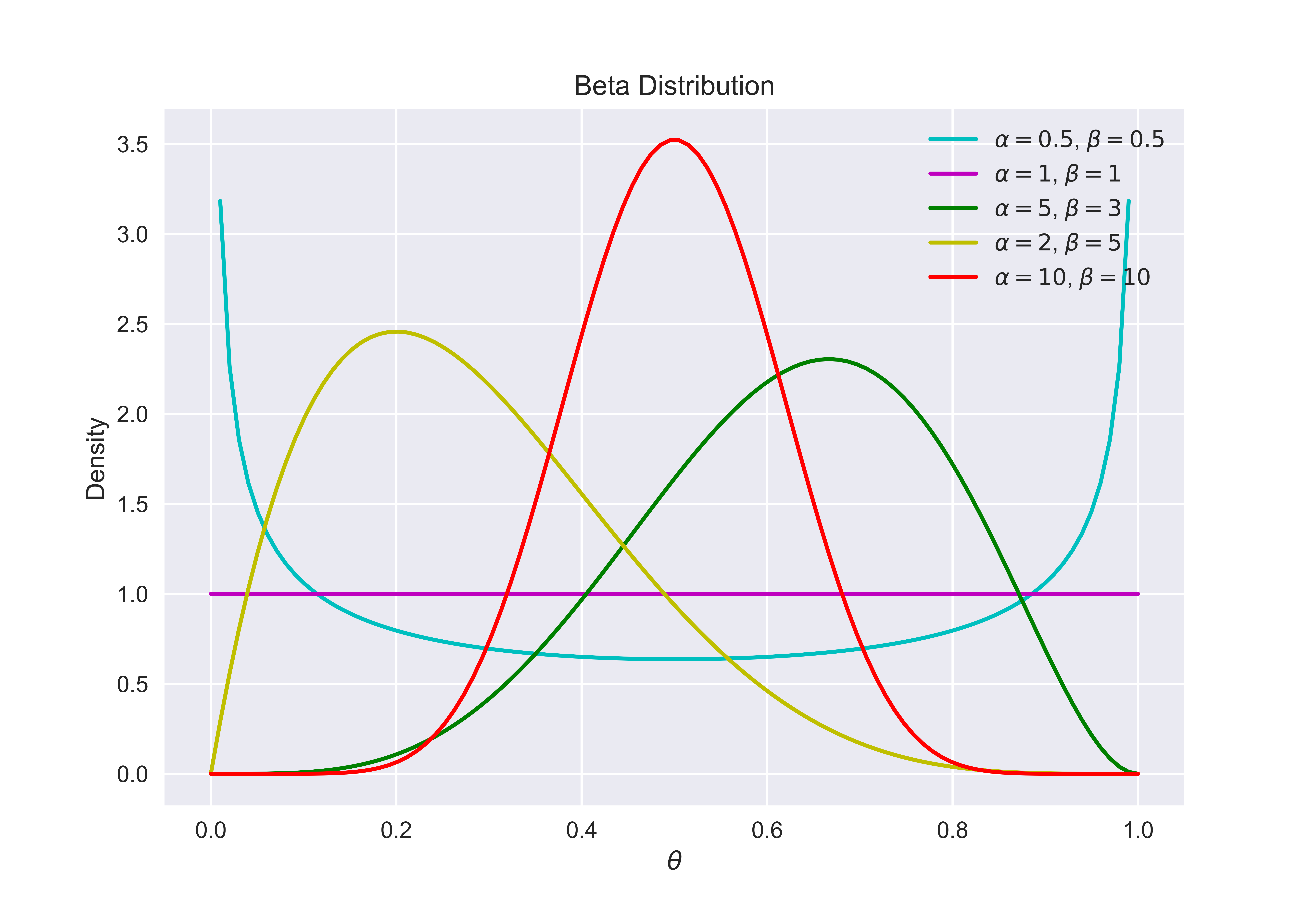
Graphically speaking, the larger the value of \(\alpha\) and \(\beta\), the more bell-shaped it becomes. Also notice that a larger \(\alpha\) corresponds to a rightward shift, i.e. a head-biased coin; a larger \(\beta\), a tail-oriented one. When \(\alpha\) and \(\beta\) take the same value, the local extrema of the Beta distribution is established at \(\theta = 0.5\), when the coin is perfectly fair.
Now that we have established the usability of the Beta function as a conjugate prior to the binomial likelihood function, let’s finally see Bayesian inference at work.
Recall the simplified version of Bayes’ theorem for inference, given as follows:
\[f(\theta \mid D) \propto L(D \mid \theta) f(\theta)\]For the prior and the likelihood, we can now plug in the equations corresponding to each distribution to generate a new posterior. Notice that \(D\), which stands for data, is now given in the form \((k, n)\) where \(k\) denotes the number of heads; \(n\), the total number of coin flips. Notice also that constants, such as the combinatorial expression or the reciprocal of the Beta function, can be dropped since we are only establishing a proportional relationship between the left and right hand sides.
\[f(\theta \mid k, n) \propto L(k, n \mid \theta) f_B(\theta; \alpha, \beta) \propto \theta^k (1 - \theta)^{n - k} \theta^{\alpha - 1} (1 - \theta)^{\beta - 1}\]Further simplifications can be applied:
\[f(\theta \mid k, n) \propto \theta^{k + \alpha - 1} (1 - \theta)^{n - k + \beta + 1}\]But notice that this expression for the posterior can be encapsulated as a Beta distribution since
\[\theta^{k + \alpha - 1} (1 - \theta)^{n - k + \beta - 1} = f_B(\theta; k + \alpha, n - k + \beta)\]Therefore, we started from a prior of \(f_B(\theta; \alpha, \beta)\) to end up with a posterior of \(f_B(\theta; k + \alpha, n - k + \beta)\). This is an incredibly powerful mechanism of updating our beliefs based on presented data. This process also proves that, as purported earlier, the Beta distribution is indeed a conjugate prior of a binomial likelihood function.
Now, it’s time to put our theory to the test with concrete numbers. Suppose we start our experiment with completely no expectation as to the fairness of the coin. In other words, the prior would appear to be a uniform distribution, which is really a specific instance of a Beta distribution with \(\alpha = \beta = 0\). Presented below is a code snippet that simulates 500 coin flips, throughout which we perform five calculations to update our posterior.
import numpy as np
import matplotlib.pyplot as plt
import seaborn as sns
from scipy import stats

n_trials = [0, 1, 2, 4, 8, 16, 32, 64, 128, 500]
data = stats.bernoulli.rvs(0.5, size=n_trials[-1])

x = np.linspace(0, 1, 100)

plt.style.use("seaborn")

for i, n in enumerate(n_trials):
	heads = data[:n].sum()

	ax = plt.subplot(len(n_trials) / 2, 2, i + 1)

	plt.setp(ax.get_yticklabels(), visible=False)

	y = stats.beta.pdf(x, heads + 1, n - heads + 1)
	plt.plot(x, y, color="skyblue", label="%d tosses,\n %d heads" % (n, heads))
	plt.fill_between(x, 0, y, color="skyblue", alpha=0.5)
	plt.legend(loc=1)

plt.tight_layout()
plt.show()
Executing this code block produces the following figure.
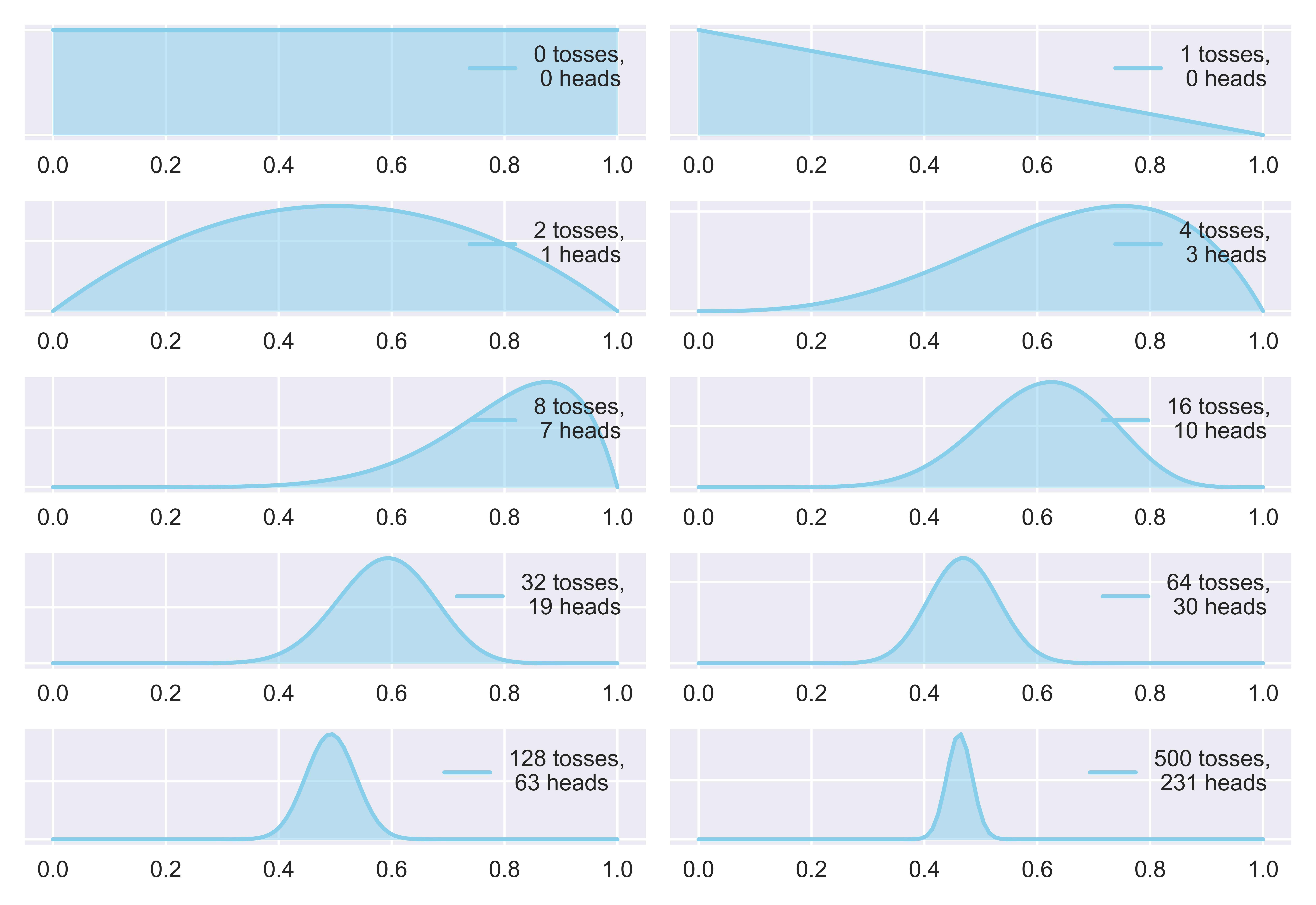
This plot shows us the change in our posterior distribution that occurs due to Bayesian update with the processing of each data chunk. Specifically, we perform this Bayesian update after [0, 1, 2, 4, 8, 16, 32, 64, 128, 500] trials. When no coin flips are performed, as shown in the first subplot, the prior follows a uniform distribution as detailed above. As more coin tosses are performed, however, we start to develop an understanding of the fairness of the coin. When we only have a few data points, the more probability there is that we obtain skewed data, which is why the mean estimate of our posterior seems skewed as well. However, with a larger number of trials, the law of large numbers guarantees that we will eventually be able to identify the value of our parameter \(\theta\), which is indeed the case.
The key takeaway from this code block is the line y = stats.beta.pdf(x, heads + 1, n - heads + 1). This is all the Bayesian method there is in this updating procedure. Notice that this line of code directly corresponds to the formula for the updated Beta posterior distribution we found earlier, which is
\(k\) refers to heads, \(n\) corresponds to n, and both \(\alpha\) and \(\beta\) are set to 1 in order to take into account the initial prior which tends to a uniform distribution. An interesting observation we can make about this result is that the variance of the Beta posterior decreases with more trials, i.e. the narrower the distribution gets. This is directly reflective of the fact that we grow increasingly confident about our estimate of the parameter with more tosses of the coin. At the end of the 500th trial, we can conclude that the coin is fair indeed, which is expected given that we simulated the coin flip using the command stats.bernoulli.rvs(0.5, size=n_trials[-1]). If we were to alter the argument for this method, say stats.bernoulli.rvs(0.7, *kwargs), then we would expect the final result of the update to reflect the coin’s bias.
Conclusion
Bayes’ theorem is a powerful tool that is the basis of Bayesian statistical analysis. Although our example was just a simple coin toss, the sample principle and mechanism can be extended to countless other situations, which is why Baye’s theorem remains highly relevant to this day, especially in the field of machine learning and statistical analysis.
Bayesian statistics presents us with an interesting way of understanding probability. The classical way of understanding probability is the frequentist approach, which purports that a probability for an event is the limit of its frequency in infinite trials. In other words, to say that a coin is fair is to say that, theoretically, performing an infinite number of coin flips would result in 50 percent heads and 50 percent tails. However, the Bayesian approach we explored today presents a drastically different picture. In Bayesian statistics, probability is an embodiment of our subjective beliefs about a parameter, such as the fairness of a coin. By performing trials, infinite or not, we gain more information about the parameter of our interest, which affects the posterior probability. Both interpretations of probability are valid, and they help complement each other to help us gain a broader understanding of what the notion of probability entails.
I hope this post gave you a better understanding as to why distributions are important—specifically in the context of conjugate priors. In a future post, we will continue our exploration of the Beta distribution introduced today, and connect the dots between Beta, Gamma, and many more distributions in the context of Bayesian statistics. See you in the next one.