Glow-TTS

Note: This blog post was completed as part of Yale’s CPSC 482: Current Topics in Applied Machine Learning.

“Turn right at 130 Prospect Street.”

If you’ve used Google maps before, you will recall the familiar, smooth voice of the navigation assistant. At first glance, the voice appears to be a simple replay of human recordings. However, you will quickly realize that it is impossible to record the names of millions of streets, not to mention the billions of driving context in which they can appear.

Modern software, such as Google maps or voice assistant, are powered by neural text-to-speech (TTS), a powerful technology that synthesize human-sounding voices using machine learning. In this blog post, we will dive deep into a NeurIPS 2020 paper Glow-TTS: A Generative Flow for Text-to-Speech via Monotonic Alignment Search, which demonstrates one of the many ways in which deep neural networks can be used for natural TTS.

Neural Text-to-Speech

Moden neural TTS pipelines are typically composed of two components: an accoustic feature generator and a vocoder. The acoustic feature generator accepts text as input and outputs an acoustic representation, such as a mel-spectrogram. The second stage of the pipeline, neural vocoders accept acoustic representations as input and outputs raw waveform. More generally, let $f$ and $g$ denote an acoustic feature generator and vocoder. Given an input text $T$, neural TTS can be understood as a composite function that outputs a waveform $W$ via

\[\begin{aligned} &X = f(T) \\ &W = g(X), \end{aligned}\]

where $X$ denotes the intermediate acoustic representation. Schematically, $g \cdot f$ fully defines the two-stage TTS process.

In this blog post, we will explore the first stage of the pipeline, the acoustic feature generator, exmplified by Glow-TTS. This post will proceed as follows. Firstly, we discuss generative flow models, which is the first core component of Glow-TTS. Secondly, we discuss the monotonic alignment search algorithm. Thirdly, we discuss the Glow-TTS pipeline as a whole by putting flow and MAS into a single picture. Last but not least, we conclude by considering some of the limitations of Glow-TTS and refer to more recent literature that points to exciting directions in the field of neural TTS.

Flow

Text-to-speech is a conditional generative task, in which a model is given a sequence of tokens and produces a stream of utterance that matches the input text. Many neural TTS models employ generative models at their core, such as GANs, VAEs, transformers, or diffision models, often borrowing from breakthroughs in other domains such as computer vision.

Change of Variables

Glow-TTS is based on normalizing flow, which is a class of well-studied generative models. The theoretical basis of normalizing flows is the change of variables formula. Let $\mathbf{X}$ and $\mathbf{Y}$ denote random variables, each with PDF $f_\mathbf{X}$ and $f_\mathbf{Y}$, respectively. Let $h$ denote some invertible transformation such that $\mathbf{Y} = h(\mathbf{X})$. Typically, $f_\mathbf{X}$ is a simple, tractable prior distribution, such as a standard Gaussian, and we seek to apply $h$ to model some more complicated distribution given by $\mathbf{Y}$. Then, the change of variables formula states that

\[\begin{aligned} f_\mathbf{Y}(\mathbf{y}) &= f_\mathbf{X}(\mathbf{x}) \bigg| \text{det} \frac{d \mathbf{x}}{d \mathbf{y}} \bigg| \\ &= f_\mathbf{X}(h^{-1}(\mathbf{y})) \bigg| \det \frac{d \mathbf{x}}{d \mathbf{y}} \bigg| \\ &= f_\mathbf{X}(h^{-1}(\mathbf{y})) \bigg| \det \frac{d h^{-1}(\mathbf{y})}{d \mathbf{y}} \bigg|, \end{aligned}\]

where $\det$ denotes the determinant and the derivative term represents the Jacobian.

A variation of this formula that allows for sampling from the base distribution can be written as follows:

\[\begin{aligned} f_\mathbf{Y}(\mathbf{y}) &= f_\mathbf{X}(\mathbf{x}) \bigg| \det \frac{d h^{-1} \mathbf{y}}{d \mathbf{y}} \bigg| \\ &= f_\mathbf{X}(\mathbf{x}) \bigg| \det \left( \frac{d h(\mathbf{x})}{d \mathbf{x}} \right)^{-1} \bigg| \\ &= f_\mathbf{X}(\mathbf{x}) \bigg| \det \frac{d h(\mathbf{x})}{d \mathbf{x}} \bigg|^{-1}. \end{aligned}\]

The intuition behind the change of variables formula is that the probability mass of an interval in $\mathbf{X}$ should remain unchanged in the transformed $\mathbf{Y}$ space. The determinant of the Jacobian is a corrective term that accounts for the slope or the “sensitivity” of the transformation given by $h$.

Maximum Likelihood

Normalizing flow models can then be understood as a collection of nested invertible transformations, i.e., $h_1 \cdot h_2 \cdots h_n$, where $n$ denotes the number of flow layers in the model.¹ To better understand what this composite transformation achieves, let’s apply a logarithm to the change of variable formula.

\[\log f_\mathbf{Y} (\mathbf{y}) = \log f_\mathbf{X} (\mathbf{x}) - \log \bigg| \det \frac{d h(\mathbf{x})}{d \mathbf{x}} \bigg|.\]

To simplify notation, let $p_i$ denote the PDF of the $i$-th random variable in the composite transformation. Then, the nested transformation can be expressed as

\[\begin{aligned} \log f_n(\mathbf{x}_n) &= \log f_{n - 1}(\mathbf{x}_{n - 1}) - \log \bigg| \det \frac{d h(\mathbf{x}_{n - 1})}{d \mathbf{x}_{n - 1}} \bigg| \\ &= \log f_{n - 2}(\mathbf{x}_{n - 2}) - \log \bigg| \det \frac{d h(\mathbf{x}_{n - 1})}{d \mathbf{x}_{n - 1}} \bigg| - \log \bigg| \det \frac{d h(\mathbf{x}_{n - 2})}{d \mathbf{x}_{n - 2}} \bigg| \\ &= \cdots \\ &= \log f_0(\mathbf{x}_0) - \sum_{i = 1}^n \log \bigg| \det \frac{d h(\mathbf{x}_i)}{d \mathbf{x}_i} \bigg|. \end{aligned}\]

The immediate implication of this exposition is that a repeated application of the change of variables formula provides a direct way of computing the likelihood of an observation from some complex, real-data distribution $f_n$ given a prior $f_0$ and a set of invertible transformation $h_1, h_2, \dots, h_n$. This conclusion illustrates the power of normalizing flows: it offers a direct way of measuring the likelihood of complex, high-dimensional data, such as ImageNet images, starting from a simple distribution, such as an isotropic Gaussian. Since the likelihood can directly be obtained, flow models are trained to maximize the log likelihood, which is exactly the expression derived above.

Affine Coupling

Although direct likelihood computation is a marked advantage of flow over other generative models, it comes with two clear limitations:

• All transformations must be invertible.
• The determinant of the Jacobian must be easily computable.

A number of methods have been proposed to satisfy these constraints. One of the most popular method is the affine coupling layer. Let $d$ denote the cardinality of the embedding space. Given an input $\mathbf{x}$ and and output $\mathbf{z}$, the affine coupling layer can schematically be written as

\[\begin{aligned} \mathbf{z}_{1:d/2} &= \mathbf{x}_{1:d/2} \\ \mathbf{z}_{d/2:d} &= \mathbf{x}_{d/2:d} \odot s_\theta(\mathbf{x}_{1:d/2}) + t_\theta(\mathbf{x}_{1:d/2}) \\ &= \mathbf{x}_{d/2:d} \odot s_\theta(\mathbf{z}_{1:d/2}) + t_\theta(\mathbf{z}_{1:d/2}). \end{aligned}\]

In other words, the affine coupling layer implements a special transformation in which the top half of $\mathbf{z}$ is simply copied from $\mathbf{x}$ without modification. The bottom half undergoes an affine transformation, where the weights and biases are computed from the top half of $\mathbf{x}$. We can easily check that this transformation is indeed invertible:

\[\begin{aligned} \mathbf{x}_{1:d/2} &= \mathbf{z}_{1:d/2} \\ \mathbf{x}_{d/2:d} &= s_\theta^{-1}(\mathbf{z}_{1:d/2})(\mathbf{z}_{d/2:d} - t_\theta(\mathbf{z}_{1:d/2})) \end{aligned}.\]

Coincidentally, the affine coupling layer is not only invertible, but it also enables efficient computation of the Jacobian determinant. This comes from the fact that the top half of the input is unchanged.

\[\begin{align} \mathbf{J} &= \begin{pmatrix} \frac{d \mathbf{z}_{1:d/2}}{d \mathbf{x}_{1:d/2}} & \frac{d \mathbf{z}_{1:2/d}}{d \mathbf{x}_{2/d:d}} \\ \frac{d \mathbf{z}_{2/d:d}}{d \mathbf{x}_{1:2/d}} & \frac{d \mathbf{z}_{d/2:d}}{d \mathbf{x}_{d/2:d}} \end{pmatrix} \\ &= \begin{pmatrix} \mathbb{I} & 0 \\ \frac{d \mathbf{z}_{2/d:d}}{d \mathbf{x}_{1:2/d}} & \text{diag}(s_\theta(\mathbf{x}_{1:d/2})) \end{pmatrix}. \end{align}\]

Although $\mathbf{J_{21}}$ contains complicated terms, we do not have to consider them when computing $\det \mathbf{J}$: the determinant of a lower triangular matrix is simply the product of its diagonal entries. Hence, $\det \mathbf{J} = \mathbf{J_{11}} \times \mathbf{J_{22}}$, which is computationally tractable.

In practice, flow layers take a slightly more complicated form than the conceptual architecture detailed above. One easy and necessary modification is to shuffle the indices that are unchanged at each layer; otherwise, the top half of the input representation would never be altered even after having passed through $n$ layers. Another sensible modification would be to apply a more complicated transformation. For example, Real NVP proposes the following schema:

\[\begin{aligned} \mathbf{z}_{1:d/2} &= \mathbf{x}_{1:d/2} \\ h &= a \times \text{tanh}(s_\theta(\mathbf{x}_{1:d/2})) + b \\ \mathbf{z}_{d/2:d} &= \text{exp}(h) \times \mathbf{x}_{d/2:d} + g_\theta(\mathbf{x}_{1:d/2}). \end{aligned}\]

To summarize:

• Flow models are based on the change of variables formula, which offers a way of understanding the PDF of the transformed random variable.
• Since flow models can directly compute the likelihood of the data distribution using a prior, it is trained to maximize the log likelihood of observed data.
• Many architectures, such as affine coupling layers, have been proposed to fulfill the invertability and Jacobian determinant constraints of flow.

Now that we have understood how flow works, let’s examine how flow is used in Glow-TTS.

Glow-TTS

Glow-TTS uses a flow-based decoder that transforms mel-spectrograms into a latent representation. As can be seen below in the architecture diagram, Glow-TTS accepts ground-truth mel-spectrograms (top of figure) and ground-truth text tokens (bottom of figure, shown as “a b c”) during training. Then, it runs the monotonic alignment search algorithm, which we will explore in the next section, to find an alignment between text and speech. The main takeaway is that the flow-based decoder transforms mel-spectrograms $\mathbf{y}$ to some latent vector $\mathbf{z}$, i.e., $f(\mathbf{y}) = \mathbf{z}$.

At a glance, it might not be immediately clear why we might want to use a flow model for the decoder instead of, for instance, a CNN or a transformer. However, the inference procedure makes clear why we need a flow-based model as the decoder. To synthesize a mel-spectrogram during inference, we estimate latent representations from user input text, then pass it on to the decoder. Since the decoder is invertible, we can reverse flow through the decoder to obtain a prediced mel-spectrogram, i.e., $f^{-1}(\hat{\mathbf{z}}) = \hat{\mathbf{y}}$, where $\hat{\cdot}$ denotes a prediction (as opposed to a ground-truth). In Glow-TTS, invertability offers an intuitive, elegant way of switching from training to inference.

The part that remains unexplained is how the model learns the latent representations and the relationship between text and acoustic features. This is explained by monotonic alignment search, which is the main topic of the next section.

Monotonic Alignment Search

Proposed by Kim et. al., Monotonic Alignment Search (MAS) is an algorithm for efficiently identifying the most likely alignment between speech and text.

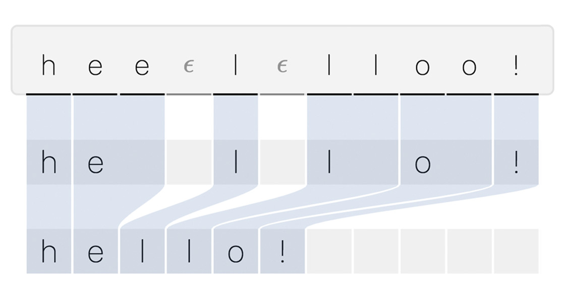
Text-to-speech alignment refers to the correspondence between text and spoken audio. Consider a simple input, “hello!”, accompanied by a human recording of that sentence. We could imagine that the first 0.5 seconds of the audio corresponds to the first letter “h,” followed by 0.7 seconds of “e,” and so on. The process of attributing a specific text token to some time interval within the audio can be described as alignment search.

Finding an accurate alignment between speech and text is an incredibly important task in TTS. If an alignment discovered by the model is inaccurate, it could mean that the model skips words or repeats certain syllables, both of which are failure nodes we want to avoid. One of the most salient features of MAS is that it prevents such failures by preemptively enforcing very specific yet sensible inductive biases into the alignment search algorithm.

Inductive Biases

Let’s begin by enumerating a list of common sense intuition we have about TTS alignments.

• The model should “read” from left to right in a linear fashion.
• The model always begins with the first letter and ends on the last letter.
• The model should not skip any text.
• The model should not repeat any text.

Many previous alignment search methods do not necessarily enforce these constraints. For instance, Tacotron 2 uses sequence-to-sequence RNN attention to autoregressively build the alignment between speech and text. However, autoregressive alignment search often fails when long input text are fed into the model since errors can accumulate throughout the text sequence, yielding a highly inaccurate alignment at the end of the iteration. On the other hand, MAS is not only non-autoregressive, but also designed specifically so that the discovered alignment will never violate the set of inductive biases outlined above. This makes the model much more robust, even when the input sequence length is arbitrairly long.

Dynamic Programming

At the heart of MAS is dynamic programming (DP), a common programming technique used to optimize runtime on problems that can be decomposed into recurring sub-problems that share the same structure as its parent. DP offers a reasonably efficient way of solving many problems, usually in $O(n^d)$ runtime, where $n$ is the size of the input and $d$ denotes DP dimensionality. While this section will not attempt to explain DP in full, we will consider a toy problem to motivate DP specifically in the context of MAS.

Consider a classic dynamic programming problem, where the goal is to find a monotonic path that maximizes the sum of scores given some score matrix. Here, “monotonic” means either moving from the current position diagonally down, or jumping to the right cell within the same row. While there might be many ways to approach this problem, here is one possible solution.

import copy

def find_maximum_sum_path(scores):
    # preliminary variables
    num_rows = len(scores)
    num_cols = len(scores[0])

    # copy to avoid overriding `scores`
    scores2 = copy.deepcopy(scores)

    # base case for first row
    for j in range(1, num_cols):
        scores2[0][j] += scores2[0][j - 1]

    # dynamic programming
    for i in range(num_rows):
        for j in range(i, num_cols):
            scores2[i][j] += max(scores2[i - 1][j - 1], scores2[i][j - 1])

    # backtracking
    # create `path` to return
    i = num_rows - 1
    path = [[0 for _ in range(num_cols)] for _ in range(num_rows)]
    for j in reversed(range(num_cols)):
        path[i][j] = 1
        if i != 0 and (i == j or scores2[i][j - 1] < scores2[i - 1][j - 1]):
            i -= 1

    return path

Given the following scores, the function returns the following result:

>>> grid = [
    [1, 3, 1, 1],
    [1, 2, 2, 2],
    [4, 2, 1, 0],
]
>>> find_maximum_sum_path(grid)
[
    [1, 1, 0, 0], 
    [0, 0, 1, 0], 
    [0, 0, 0, 1]
]

It is not difficult to perform a manual sanity to check that the returned result is indeed the path that maximizes the sum of scores while adhering to the monotonicity constraint.

Likelihood Scores

Let’s take a step back and revisit the model architecture diagram presented above. On the left side of the diagram, we see an illustration of monotonic alignment search in action. Notice that this is exactly the problem we solved above: given some matrix of scores, find a monotonic path that maximizes the sum. Now, only a few missing pieces remain:

• What is the matrix of scores?
• How does this relate to the flow-based decoder?

Turns out that the two questions are closely related, and answering one will shed light on the other.

Recall that Glow-TTS deals with two input modalities during training: a string of text and its corresponding mel-spectrogram. The mel-spectrogram is decoded through the flow-based decoder. Similarly, the text is fed to a text encoder network, which outputs $\mathbf{\mu}$ and $\mathbf{\sigma}$ for each token of text. In other words, given ["h", "e", "l", "l", "o"], we would have a total of five mean and standard deviation vectors corresponding to each letter.² We can denote them as $\mathbf{\mu_1}, \mathbf{\mu_2}, \dots, \mathbf{\mu_5}$, and $\mathbf{\sigma_1}, \mathbf{\sigma_2}, \dots, \mathbf{\sigma_5}$. Let’s also assume in this example that the corresponding mel-spectrogram spans a total of 100 frames. The output of the flow decoder would also be 100 vectors, denoted as $\mathbf{z_1}, \mathbf{z_2}, \dots, \mathbf{z_{100}}$.

Using these quantities, we can then construct a likelihood score matrix $P \in \mathbb{R}^{5 \times 100}$. The entries of the probability score matrix are computed via $P_{ij} = \log(\phi(\mathbf{z_j}; \mu_i, \sigma_i))$, where $\phi$ denotes the normal probability density function. Since $\sigma$ is a vector instead of a matrix, we assume an isotropic Gaussian, i.e., the covariance matrix is diagonal. The intuition is that the value of $P_{ij}$ indicates how likely it is that the $i$-th character matches or aligns with the $j$-th mel-spectrogram frame. If the two pairs of text and audio match, the probability score will be high, and vice versa. Log likelihood is used so that summation of scores effectively models a product in probability space.

Given this context, we can now apply the solution to the monotonic path sum problem motivated in the previous section. Instead of some arbitrary scores matrix, we create the probability score matrix $P$ and use DP to discover the most likely monotonic alignment between speech and text. The alignment will satisfy the inductive biases we identified earlier due to the inherent design of MAS.

It is worth noting that MAS is a generic alignment search algorithm that is independent of the flow-based model design. In particular, MAS was used without the flow decoder in Grad-TTS. Popov et. al. proposed using mel-spectrogram frames directly to measure the probability score given the mean and variance prediced from text. In other words, instead of using $\mathbf{z}$, mel-spectrogram frames $\mathbf{y}$ were used. Grad-TTS is notable in its use of score-based generative models, which fall under the larger category of diffusion-based probabilistic models.

Glow-TTS Pipeline

We can finally put flow and MAS together to summarize the overall pipeline of Glow-TTS.

Training

Given a pair of text and mel-spectrogram $(T, \mathbf{y})$, we feed $T$ into the text encoder $f_\text{text}$ and mel-spectrogram $\mathbf{y}$ into the flow-based decoder $f_\text{mel}$ to obtain $f_\text{mel}(\mathbf{y}) \in \mathbb{R}^{D \times L_\text{mel}}$ and $f_\text{text}(T) = (\mu, \sigma)$, where $\mu, \sigma \in \mathbb{R}^{D \times L_\text{text}}$ and $D$ denotes the size of the embedding. We can then use MAS to obtain the most likely monotonic alignment $A^* \in \mathbb{R}^{L_\text{text} \times L_\text{mel}}$. Since Glow-TTS is a flow-based model, which enables direct computation of likelihood, the model is simply trained to maximize the value of the log-likelihood given by the sum of the entries of the log-likelihood score matrix $P$. $A^\star$ can intuitively be understood as a binary mask used to index $P$. Schematically, the final log-likelihood could be written as $l = \sum_{i = 1}^{L_\text{text}} \sum_{j = 1}^{L_\text{mel}}(P \odot A^\star)_{ij}$, where $\odot$ denotes a Hadamard product, or an element-wise product of matrices. Since optimization in modern machine learning are typically framed as a minimizing problems, we minimize the negative log-likelihood.

Although not discussed in the sections above, Glow-TTS requires training a small sub-model, called a duration predictor, for inference. Because we do not have access to the ground-truth mel-spectrogram during inference, we need a model that can predict the best alignment $A^*$ purely from text. This task is carried out by the duration predictor, which accepts $T$ as input and is trained to maximize the L2 distance between its predicted alignment $\hat{A}$ and the actual $A^\star$ discovered by MAS.

Inference

In the context of inference, the model has to output a predicted mel-spectrogram $\hat{\mathbf{y}}$ conditioned on the input text $T$. First, we use the learned text encoder to obtain mean and variance, i.e., $f_\text{text}(T) = (\mu, \sigma)$. Then, we use the duration predictor to obtain a predicted alignment $\hat{A}$. We can then sample from the $\mathcal{N}(\mu, \sigma^2)$ distribution according to $\hat{A}$. Continuing the earlier example of T = ["h", "e", "l", "l", "o"], let’s say that A_star = [1, 3, 2, 1, 1]. This means that we have to sample from $\mathcal{N}(\mu_\text{h}, \sigma_\text{h})$ once, $\mathcal{N}(\mu_\text{e}, \sigma_\text{e})$ three times, and so on. By concatenating the results of sampling, we obtain $\hat{\mathbf{z}} \in \mathbb{R}^{D \times \hat{L_\text{mel}}}$, where $\hat{L_\text{mel}}$ denotes the length of the predicted mel-spectrogram frames, which is effectively sum(A_star). Once we have $\hat{\mathbf{z}}$, we finally use the flow decoder to invert it into the mel-spectrogram space, i.e., $f_\text{mel}^{-1}(\hat{\mathbf{z}}) = \hat{\mathbf{y}}$.

Sample diversity is an important concern in neural TTS. Just like humans can read a single sentence in many different ways by varying tone, pitch, and timbre, preferably, we want a TTS model to be able to produce diverse samples. One way to achieve this in Glow-TTS is by varying the temperature parameter during sampling. In practice, sampling is performed thorugh the reparametrization trick:

\[\epsilon \sim \mathcal{N}(0, 1) \\ \mathbf{z} = \mu + \epsilon \cdot \sigma^2.\]

Through listening tests and pitch contours, Kim et. al. show that varying $\epsilon$ achieves diversity among samples produced by Glow-TTS.

Results

A marked advantage of Glow-TTS is that it is a parallel TTS model. This contrasts with existing autoregressive baselines, such as Tacotron 2. While autoregressive models require an iterative loop to condition the output of the current timestep on that from the previous timestep, parallel models produce an output in a single pass. In other words, parallel models run in constant time, whereas the runtime complexity of autoregressive models scales linearly with respect to the length of the input sequence. This is clear in the comparison figure taken from the Glow-TTS paper.

Another pitfall of autoregressive models is that errors can accumulate throughout the iterative loop. If the model misidentifies an alignment between speech and text early on in the input sequence, later alignments will also likely be incorrect. In the case of parallel models, error accumulation is not possible since there is no iterative loop to begin with. Moreover, alignments found by Glow-TTS are made even more robust due to the design of MAS, which systematically identifies only those alignments that satisfy the monotonicity inductive bias. In the figure below, also taken directly from the Glow-TTS paper, Kim et. al. show that the Glow-TTS maintains a consistent character error rate, while that of Tacotron 2 increases proportionally to the length of the input sequence.

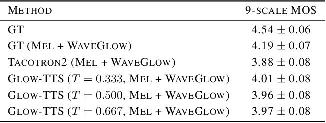
Glow-TTS achieves competitive results on mean opnion score (MOS) listening tests. MOS tests are typically performed by randomly sampling a number of people and providing them to rate an audio sample from a scale of 1 to 5, where higher is better.

In the results table shown below, GT (ground-truth) is rated most highly at 4.54. WaveGlow is a neural vocoder that transforms mel-spectrograms to waveform. GT (Mel + WaveGlow) received 4.19, marginally below the GT waveform score. This is because using a neural vocoder necessarily introduces quality degradations and artifacts. Since even the best neural TTS acoustic feature generator would not be able to produce a mel-spectrogram that sounds more natural than a human recording, 4.19 can be considered as the theoretical upperbound for any TTS model and WaveGlow combination. Glow-TTS comes pretty close to 4.19, scoring approximately 4 across various temperature parameters. While the difference of 0.19 certainly suggests room for improvement, it is worth mentioning that Glow-TTS outperforms the Tacotron 2, which has been considered the competitive SOTA TTS model for a long time.

Future Direction

An emerging trend in neural TTS literature is end-to-end TTS modeling. Instead of the traditional two-stage pipeline composed of an acoustic feature generator and a neural vocoder, end-to-end models produce raw waveforms directly from text without going to the intermediate mel-spectral representation. One prime example is VITS, an end-to-end speech model developed by the authors of Glow-TTS published in ICML 2021. VITS is a combination of Glow-TTS and HiFi-GAN, which is a neuarl vocoder. VITS uses largely the same MAS algorithm as Glow-TTS, and uses a variational autoencoding training scheme to combine the feature generator and the neural vocoder.

A benefit of using end-to-end modeling is that the model is relieved of the mel-spectral information bottleneck. Mel-spectrogram is a specific representation of information defined and crafted according to human knowledge. However, the spirit of deep learning is that no manual hand-crafting of features is necessary, provided sufficient data and modeling capacity. End-to-end models allow the model to choose its own intermediate representation that best accomplishes the task of synthesizing natural-sounding audio. Indeed, VITS outperforms Tacotron and Glow-TTS by considerable margins and almost matches ground-truth MOS ratings. This is certainly an exciting development, and we can expect more lines of work in this direction.

Conclusion

Glow-TTS is a flow-based neural TTS model that demonstrated a method of leveraging the invertability of flow to produce mel-spectrograms from text-derived latent representations. By projecting mel-spectrograms and text into a common latent space and using MAS and maximum likelihood-based training, Glow-TTS is able to learn robust, hard monotonic alignments between speech and text. Similar to Tacotron 2, Glow-TTS is now considered a competitive baseline and is referenced in recent literature.

Neural TTS has seen exciting developments over the past few years, including general text-to-speech, voice cloning, singing voice synthesis, and prosody transfer. Moreover, given the rapid pace of development in other fields, such as natural language processing, automatic speech recognition, and multidmodal modeling, we could see more interesting models that combine different approaches and modalities to perform a wide array of complex tasks. If anything remains clear, it is that we are living at an exciting time in the era of machine learning, and that the next few years will continue to see breakthroughs and innovations that will awe and surprise us, just like people a few decades ago would marvel at the simplest words:

“Turn right at 130 Prospect Street.”

1. While there are variations of normalizing flows, such as continuous flows or neural ODEs, for sake of simplicity, we only consider discontinuous normalizing flow. ↩

2. In practice, most TTS models, including Glow-TTS, use phonemes as input instead of characters of text. We illustrate the example using characters for simplicity. ↩