0.5!: Gamma Function, Distribution, and More

In a previous post, we looked at the Poisson distribution as a way of modeling the probability of some event’s occurrence within a specified time frame. Specifically, we took the example of phone calls and calculated how lucky I was on the day I got only five calls during my shift, as opposed to the typical twelve.

While we clearly established the fact that the Poisson distribution was a more accurate representation of the situation than the binomial distribution, we ran into a problem at the end of the post: how can we derive or integrate the Poisson probability distribution, which is discontinuous? To recap, let’s reexamine the Poisson distribution function:

\[P(X = k) = \lim\limits_{n \to \infty} e^{- \lambda} \frac{\lambda^k}{k!}\]

As you can see, this function is discontinuous because of that one factorial term shamelessly flaunting itself in the denominator. The factorial, we might recall, is as an operation is only defined for integers. Therefore, although we can calculate expression such as \(7!\), we have no idea what the expression \(0.5!\) evaluates to.

Or do we?

Here is where the Gamma function kicks in. This is going to be the crux of today’s post.

The Gamma Function

Let’s jump right into it by analyzing the Gamma function, specifically Euler’s integral of the second kind:

\[\Gamma(n + 1) = \int_0^\infty x^n e^{-x} \, dx\]

At a glance, it is not immediately clear as to why this integral is an interpolation of the factorial function. However, if we try to evaluate this expression through integration by parts, the picture becomes clearer:

\[\int_0^\infty x^n e^{-x} \, dx = - x^n e^{-x} \Big|_{0}^{\infty} + n \int_0^\infty x^{n - 1} e^{-x} \, dx\]

Notice that the first term evaluates to 0. Moreover, the integral term can be expressed in terms of the Gamma function since

\[\int_0^\infty x^{n - 1} e^{-x} \, dx = \Gamma(n - 1)\]

Applying all the simplifications leave us with

\[\Gamma(n + 1) = n\Gamma(n)\]

Notice that this is a recursive representation of the factorial, since we can further unravel \(\Gamma(n)\) using the same definition. In other words,

\[\Gamma(n + 1) = n \cdot (n - 1) \cdot (n - 2) \cdot \dots \cdot 1 = n!\]

So it is now clear that the Gamma function is indeed an interpolation of the factorial function. But the Gamma function deserves a bit more attention and analysis than the simple evaluation we have performed above. Specifically, I want to introduce a few more alternative forms of expressing and deriving the Gamma function. There are many ways to approach this subject, and it would be impossible to exhaust through the entire list of possible representations. For the purposes of this post, we look at two forms of the Gamma function I find intriguing.

The first version, presented below, is Euler’s definition of the Gamma function as an infinite product.

\[\Gamma(x) = \lim\limits_{n \to \infty} \frac{n^x n!}{x(x + 1)(x + 2) \dots (x + n)}\]

To see how this comes from, we backtrack this equality by dividing the right-hand side by \((x - 1)!\).

\[\lim\limits_{n \to \infty} \frac{n^x n!}{x(x + 1)(x + 2) \dots (x + n) \cdot (x - 1)!} = \lim\limits_{n \to \infty} \frac{n^x n!}{(x + n)!} = 1\]

At this point, we can reduce the fraction by eliminating \(n!\) from both the denominator and the numerator, which leaves us with the following expression:

\[\lim\limits_{n \to \infty} \frac{n^x}{(n + 1)(n + 2) \dots (n + x)} = \lim\limits_{n \to \infty} \frac{n}{(n + 1)} \frac{n}{(n + 2)} \dots \frac{n}{(n + x)} = 1\]

Therefore, we have

\[(x - 1)! = \Gamma(x) = \lim\limits_{n \to \infty} \frac{n^x n!}{x(x + 1)(x + 2) \dots (x + n)}\]

This is another representation of the Gamma function that is distinct from the integral we saw earlier. The last form that we will see involves some tweaking of the harmonic series, or the simplest case of the Riemann zeta function where \(s = 1\). We start from \(\log x!\).

\[f(x) = \ln x! = \ln x + \ln (x - 1)! = \ln x + f(x - 1)\]

We derive both sides by \(x\) to obtain the following:

\[f'(x) = \frac{1}{x} + f'(x - 1) = \frac{1}{x} + \frac{1}{x - 1} \dots \frac{1}{1} + f'(0)\]

Notice the harmonic series embedded in the expression above. To further simplify this expression, we derive an interpolation of the harmonic series. Let the interpolation be denoted as \(g(n)\):

\[g(n) = t + \frac{1}{2}t^2 + \dots + \frac{1}{n}t^n\]

We derive both sides by \(t\) to obtain the following:

\[\frac{d[g(n)]}{dt} = g'(n) = 1 + t + \dots + t^{n - 1}\]

The expression above is the sum of a geometric series with radius \(t\).

\[g'(n) = \frac{1 - t^n}{1 - t}\]

We integrate both sides by \(n\) to obtain \(g(n)\).

\[\int g'(n) \, dn = g(n) = \int \frac{1 - t^n}{1 - t} \, dn\]

We are almost done! Now that we have the expression for the harmonic series, we can plug it back into the original equation on \(f(x)\) to finish off this derivation.

\[f'(x) = \frac{1}{x} + \frac{1}{x - 1} + \dots + \frac{1}{1} + f'(0) = \int_0^1 \frac{1 - t^n}{1 - t} + f'(0) \, dn\]

Integrate both sides by \(x\) to obtain the following:

\[f(x) = \ln x! = \int_0^x \int_0^1 \frac{1 - t^n}{1 - t} + f'(0) \, dn \, dx\]

Exponentiate both sides by \(e\) to remove the logarithm, and we finally get the alternative representation of the Gamma function:

\[e^{\ln x!} = x! = \Gamma(x - 1) = e^{\int_0^x \int_0^1 \frac{1 - t^n}{1 - t} + f'(0) \, dn \, dx}\]

So we see that there are many other alternate modes of expressing the same function, \(\Gamma(n)\). But the truth that remains unchanged is that the Gamma function is essentially a more expansive definition of the factorial that allows for operations on any real numbers. There are many concepts and theories surrounding the Gamma function, such as the Euler-Mascheroni constant, Mellin transformation, and countless many more, but these might be tabled for another discussion as they each deserve a separate post.

The Gamma Distribution

The Gamma distribution is, just like the binomial and Poisson distribution we saw earlier, ways of modeling the distribution of some random variable \(X\). Deriving the probability density function of the Gamma distribution is fairly simple. We start with two parameters, \(\alpha > 0\) and \(\beta > 0\), using which we can construct a Gamma function.

\[\Gamma(\alpha) = \int_0^\infty x^{\alpha - 1} e^{-x} \, dx\]

We can divide both sides by \(\Gamma(\alpha)\) to obtain the following expression:

\[1 = \frac{\int_0^\infty x^{\alpha - 1} e^{-x} \, dx} {\Gamma(\alpha)}\]

We can then apply the substitution \(x = \beta y\) to obtain

\[1 = \frac{\int_0^\infty \beta^\alpha y^{\alpha - 1} e^{-\beta y} \, dy}{\Gamma(\alpha)}\]

Notice that we can consider the integrand to be a probability distribution function since the result of integration over the prescribed domain yields 1, the total probability. Seen this way, we can finally delineate a definition of the Gamma distribution as follows, with a trivial substitution of parameters.

\[P(T = k; \alpha, \beta) = \frac{\beta^\alpha k^{\alpha - 1} e^{-\beta k}}{\Gamma(\alpha)}\]

If this derivation involving the Gamma function does not click with you, we can take the alternative route of starting from the functional definition of the Gamma distribution: the Gamma distribution models the waiting time until the occurrence of the \(k\)th event in a Poisson process. In other words, given some rate \(\lambda\) which denotes the rate at which an event occurs, what is the distribution of the waiting time going to look like? The Gamma distribution holds an answer to this question.

Let’s jump right into derivation. The first ingredient we need is the equation for the Poisson probability mass function, which we might recall goes as follows:

\[P(X = k) = \frac{\lambda^k e^{-\lambda}}{k!}\]

\(k\) denotes the number of events that occur in unit time, while \(\lambda\) denotes the rate of success. To generalize this formula by removing the unit time constraint, we can perform a rescaling on \(\lambda\) to produce the following:

\[P(X = k) = \frac{(\lambda t)^k e^{-\lambda t}}{k!}\]

where \(P(X = k)\) denotes the probability that \(k\) events occur within time \(t\). Notice that setting \(t = 1\) gives us the unit time version of the formula presented above.

The link between the Poisson and Gamma distribution, then, is conveniently established by the fact that the time of the \(k\)th arrival is lesser than \(t\) if more than \(k\) events happen within the time interval \([0, t]\). This proposition can be expressed as an identity in the following form.

\[F(t) = P(T < t) = \sum_{x = k}^{\infty} \frac{(\lambda t)^x e^{-\lambda t}}{x!}\]

Notice that the left-hand side is a cumulative distribution function of the Gamma distribution expressed in terms of \(t\). Given the derivative relationship between the CDF and PDF, we can obtain the probability distribution function of Gamma by deriving the right-hand side sigma expression with respect to \(t\).

\[F’(t) = f(t) = {\sum_{x = k}^\infty \lambda \frac{(\lambda t)^{x - 1}}{(x - 1)!} e^{- \lambda t}} - {\sum_{x = k}^\infty \lambda \frac{(\lambda t)^x}{x!} e^{- \lambda t}}\]

After some thinking, we can convince ourselves that unraveling the sigma results in a chain reaction wherein adjacent terms nicely cancel one another, ultimately collapsing into a single term, which also happens to be the first term of the expression:

\[f(t) = \lambda \frac{(\lambda t)^{k - 1}}{(k - 1)!} e^{- \lambda t} - \lambda \frac{(\lambda t)^k}{k!} e^{- \lambda t} + \lambda \frac{(\lambda t)^k}{k!} e^{- \lambda t} + \dots = \lambda \frac{(\lambda t)^{k - 1}}{(k - 1)!} e^{- \lambda t}\]

Recalling that \(\Gamma(k) = (k - 1)!\), we can rewrite the expression as follows:

\[f(t) = \lambda \frac{(\lambda t)^{k - 1}}{\Gamma(k)} e^{- \lambda t} = \frac{\lambda^k t^{k - 1} e^{- \lambda t}}{\Gamma(k)}\]

Notice the structural identity between the form we have derived and the equation of the Gamma distribution function introduced above, with parameters \(\alpha\), \(\beta\), and \(k\). In the language of Poisson, these variables translate to \(k\), \(\lambda\), and \(t\), respectively.

To develop and intuition of the Gamma distribution, let’s quickly plot the function. If we determine the values for the parameters \(\alpha\) and \(\beta\), the term \(\beta^\alpha/\Gamma(\alpha)\) reduces to some constant, say \(C\), allowing us to reduce the PDF into the following form:

\[f(k) = C k^{\alpha - 1} e^{- \beta k}\]

This simplified expression reveals the underlying structure behind the Gamma distribution: a fight for dominance between two terms, one that grows polynomially and the other that decays exponentially. Plotting the Gamma distribution for different values of \(\alpha\) and \(\beta\) gives us a better idea of what this relationship entails.

import numpy as np
import matplotlib.pyplot as plt
import seaborn as sns
from scipy.stats import gamma

plt.style.use("seaborn")
x = np.linspace (0, 50, 200)
y1 = gamma.pdf(x, a=1, loc=10)
y2 = gamma.pdf(x, a=3, loc=10)
y3 = gamma.pdf(x, a=5, loc=10)
y4 = gamma.pdf(x, a=10, loc=10)
y5 = gamma.pdf(x, a=5, loc=30)
plt.xlabel('X')
plt.ylabel('P(X)')
plt.title('Gamma Distribution')
plt.grid(True)
plt.plot(x, y1, "c-", label=(r'$\\alpha=1, \\beta=10$'))
plt.plot(x, y2, "m-", label=(r'$\\alpha=3, \\beta=10$'))
plt.plot(x, y3, "g-", label=(r'$\\alpha=5, \\beta=10$'))
plt.plot(x, y4, "y-", label=(r'$\\alpha=10, \\beta=10$'))
plt.plot(x, y5, "r-", label=(r'$\\alpha=5, \\beta=30$'))
plt.legend()
plt.ylim([0,1])
plt.xlim([5,45])
plt.show()

Executing this code block produces the following figure.

Figure 1: Gamma distribution for different parameters

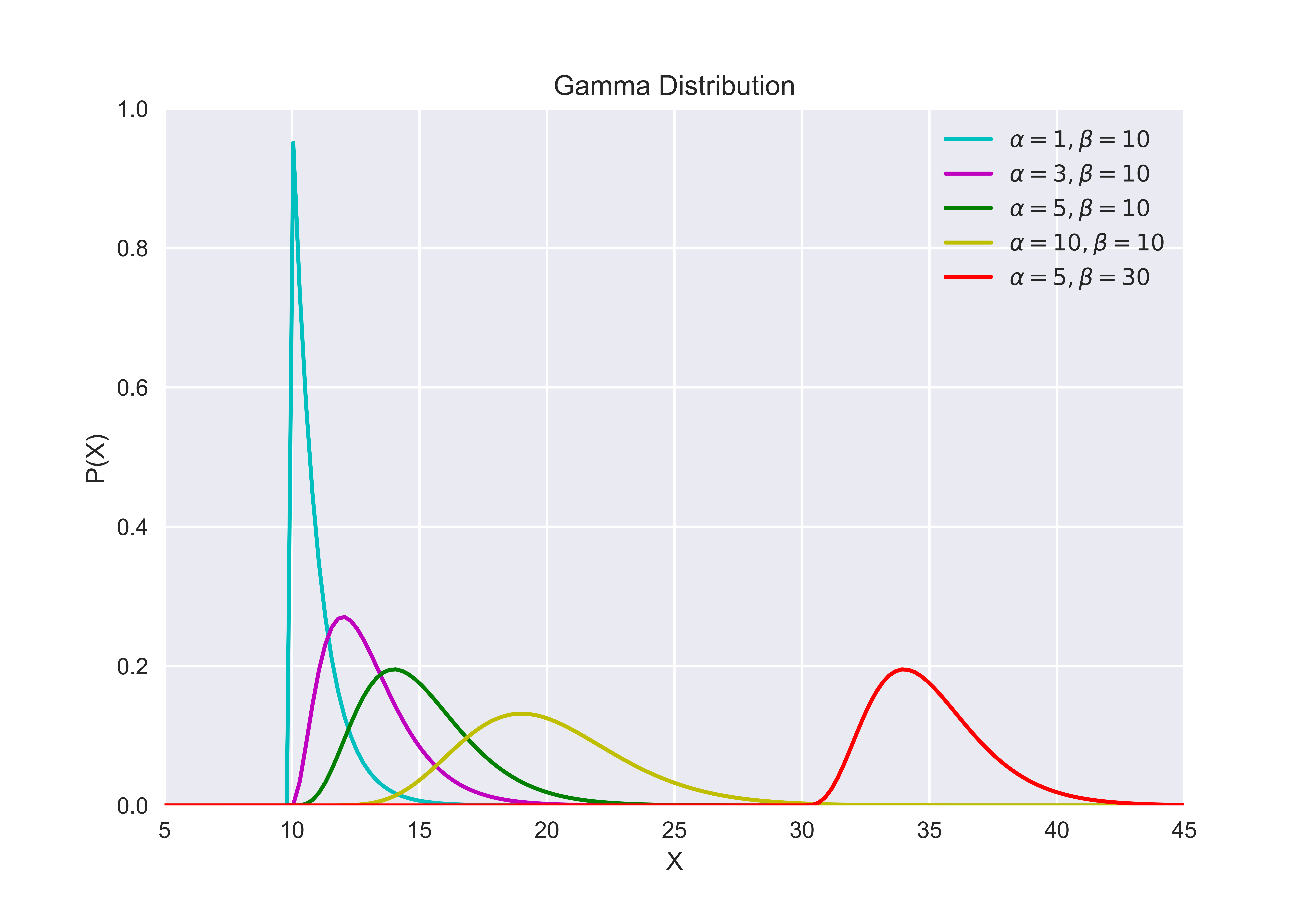
Notice that, as \(\alpha\) increases, the Gamma distribution starts to look more like a normal distribution. At \(\alpha = 1\), the \(k^{a - 1}\) collapses to 1, resulting in an exponential distribution. A short tangential digression: the exponential distribution is a special case of a Gamma distribution that models the waiting time until the first event in a Poisson process. It can also be considered as the continuous version of the geometric distribution. But maybe more on this later on a separate post.

Returning back to the Gamma distribution, we see that altering the \(\beta\) also produces a transformative effect on the shape of the Gamma PDF. Specifically, increasing \(\beta\) causes the distribution to move to the right along the \(x\)-axis. This movement occurs because, for every \(x\), a larger \(\beta\) value results in a decrease in the corresponding value of \(P(X = x)\), which graphically translates to a rightward movement along the axis as shown.

Conclusion

We started by looking at the Poisson probability mass function, and started our venture into the Gamma function by pondering the question of interpolating the factorial function. From there, we were able to derive and develop an intuition for the Gamma distribution, which models the waiting time required until the occurrence of the \(k\)th event in a Poisson process.

This may all sound very abstract because of the theoretical nature of our discussion. So in the posts to follow, we will explore how these distributions can be applied in different contexts. Specifically, we will take a look at Bayesian statistics and inference to demonstrate how distributions can be employed to express prior or posterior probabilities. At the same time, we will also continue our exploration of the distribution world by diving deeper into other probability distributions, such as but not limited to exponential, chi-square, normal, and beta distributions, in no specific order. At the end of the journey, we will see how these distributions are all beautifully interrelated.

Catch you up in the next one!