How lucky was I on my shift?
At the Yongsan Provost Marshall Office, I receive a wide variety of calls during my shift. Some of them are part of routine communications, such as gate checks or facility operation checks. Others are more spontaneous; fire alarm reports come in from time to time, along with calls from the Korean National Police about intoxicated soldiers who get involved in mutual assault or misdemeanors of the likes. Once, I got a call from the American Red Cross about a suicidal attempt of a soldier off post. All combined, I typically find myself answering about ten to fifteen calls per shift.
But yesterday was a special day, a good one indeed, because I received only five calls in total. This not only meant that USAG-Yongsan was safe and sound, but also that I had a relatively light workload. On other days when lawlessness prevails over order, the PMO quickly descends into chaos—patrols get dispatched, the desk sergeant files mountains of paperwork, and I find myself responding to countless phone calls while relaying relevant information to senior officials, first sergeants, and the Korean National Police.
So yesterday got me thinking: what is the probability that I get only five calls within a time frame of eight hours, given some estimate of the average number of calls received by the PMO, say 12? How lucky was I?
The Binomial Distribution
One way we might represent this situation is through a binomial distribution. Simply put, a binomial distribution simulates multiple Bernoulli trials, which are experiments with only two discrete results, such as heads and tails, or more generally, successes and failures. A binomial random variable \(X\) can be defined as the number of success in \(n\) repeated trials with probability of success \(p\). For example, if we perform ten tosses of a fair coin, the random variable would be the number of heads; \(p\) would be \(0.5\), and \(n\) would be \(10\).
Mathematically, the probability distribution function of a binomial distribution can be written as follows:
\[P(X = k) = \binom{n}{k} p^k (1 - p)^{n - k}\]We can derive this equation by running a simple thought experiment. Let’s say we are tossing a coin ten times. How can we obtain the probability of getting one head and nine tails? To begin with, here is the list of all possible arrangements:
[['H', 'T', 'T', 'T', 'T', 'T', 'T', 'T', 'T', 'T'],
['T', 'H', 'T', 'T', 'T', 'T', 'T', 'T', 'T', 'T'],
['T', 'T', 'H', 'T', 'T', 'T', 'T', 'T', 'T', 'T'],
['T', 'T', 'T', 'H', 'T', 'T', 'T', 'T', 'T', 'T'],
['T', 'T', 'T', 'T', 'H', 'T', 'T', 'T', 'T', 'T'],
['T', 'T', 'T', 'T', 'T', 'H', 'T', 'T', 'T', 'T'],
['T', 'T', 'T', 'T', 'T', 'T', 'H', 'T', 'T', 'T'],
['T', 'T', 'T', 'T', 'T', 'T', 'T', 'H', 'T', 'T'],
['T', 'T', 'T', 'T', 'T', 'T', 'T', 'T', 'H', 'T'],
['T', 'T', 'T', 'T', 'T', 'T', 'T', 'T', 'T', 'H']]
Notice that all we had to do was to choose one number \(i\) that specifies the index of the trial in which a coin toss produced a head. Because there are ten ways of choosing a number from integers \(1\) to \(10\), we got ten different arrangements of the situation satisfying the condition \(X_{head} = 1\). You might recall that this combinatoric condition can be expressed as \(\binom{10}{1}\), which is the coefficient of the binomial distribution equation.
Now that we know that there are ten different cases, we have to evaluate the probability that each of these cases occur, since the total probability \(P(X_{head} = 1) = \sum_{n=1}^{10} p_i = 10 \cdot p_i\), where \(p_i\). Calculating this probability is simple: take the first case, ['H', 'T', 'T', 'T', 'T', 'T', 'T', 'T', 'T', 'T'] as an example. Assuming independence on each coin toss, we can use multiplication to calculate this probability:
Notice that \(p = 1 - p = \frac12\) because we assumed the coin was fair. Had it not been fair, we would have different probabilities for \(p_{success}\) and \(p_{fail}\), explained by the relationship that \(p_{success} + p_{fail} = 1\). This is what the binomial PMF is implying: calculating the probability that we get \(k\) successes in \(n\) trials requires that we multiply the probability of success \(p\) by \(k\) times and the probability of failure \((1 - p)\) by \((n - k)\) times, because those are the numbers of successful and unsuccessful trials respectively.
Now that we have reviewed the concept of binomial distribution, it is time to apply it to our example of phone calls at the Yongsan PMO. Although I do not have an .csv data sheet on me, let’s assume for the sake of convenience that, on average, 12 calls come to the PMO per shift, which is eight hours. Given this information, how can we simulate the situation as a binomial distribution?
First, we have to define what constitutes a success in this situation. While there might be other ways to go about this agenda, the most straightforward approach would be to define a phone call as a success. This brings us to the next question: how many trials do we have? Here is where things get a bit more complicated—we don’t really have trials! Notice that this situation is somewhat distinct from coin tosses, as we do not have a clearly defined “trial” or an experiment. Nonetheless, we can approximate the distribution of this random variable by considering each ten-minute blocks as a unit for a single trial, i.e. if a call is received by the PMO between 22:00 and 22:10, then the trial is a success; if not, a failure. Blocking eight hours by ten minutes gives us a total of 48 trials. Because we assumed the average number of phone calls on a single shift to be 12, the probability of success \(p = 0.25\).
Let’s simulate this experiment \(10000\) times. We can model this binomial distribution as follows:
from scipy.stats import binom
import matplotlib.pyplot as plt
import seaborn as sns

plt.style.use("seaborn")

data_binom = binom.rvs(n=48,p=0.25,size=10000)

ax = sns.distplot(data_binom,
                  kde=False,
                  color='skyblue',
                  hist_kws={"linewidth": 15,'alpha':1})

plt.xlabel('X')
plt.ylabel('P(X)')
plt.title('Binomial Probability Distribution')
plt.grid(True)
plt.show()
This code block produces the following output:
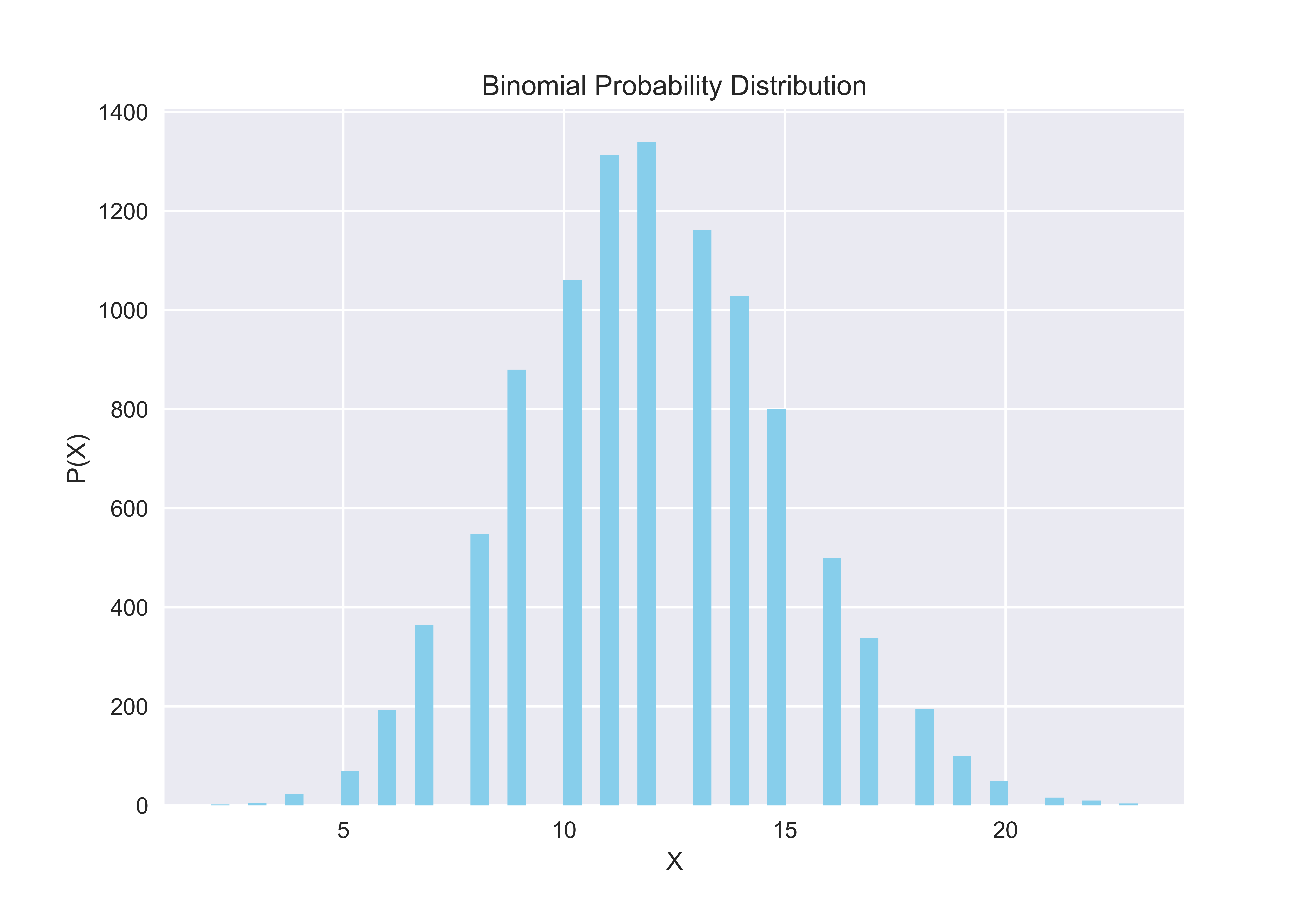
Under this assumption, we can also calculate how lucky I was yesterday when I only received five calls by plugging in the appropriate values into the binomial PMF function:
\[P(X = 5) = \binom{48}{5} \cdot 0.25^5 \cdot 0.75^{43} = 1712304 \cdot 9.765625 \cdot 10^{-4} \cdot 4.24262 \cdot 10^{-6} \approx 0.0071\]From a frequentist’s point of view, I would have lazy days like these only 7 times for every thousand days, which is nearly three years! Given that my military service will last only 1.5 years from now, I won’t every have such a lucky day again, at least according to the binomial distribution.
But a few glaring problem exists with this mode of analysis. For one, we operated under a rather shaky definition of a trial by arbitrarily segmenting eight hours into ten-minute blocks. If we modify this definition, say, by saying that a single minute comprises an experiment, hence a total of 480 trials, we get a different values for \(n\) and \(p\), which would clearly impact our calculation of \(P(X = 5)\). In fact, some weird things happen if we block time into large units, such as an hour—notice how the value of \(p\) becomes \(12/8 = 1.5\), which is a probabilistic impossibility as \(p\) should always take values between \([0, 1]\).
Another issue with this model is that a Bernoulli trial does not allow for simultaneous successes. Say, for instance, that within one ten-minute block, we got two calls. However, because the result of a Bernoulli trial is binary, i.e. either a success or a failure, it cannot contain more than one success in unit time. Therefore, binary distribution cannot encode higher dimensions of information, such as two or three simultaneous successes in one trial.
These set of complications motivate a new way of modeling phone calls. In the next section, we look at an alternate approach to the problem: the Poisson distribution.
The Poisson Distribution
Here is some food for thought: what if we divide up unit time into infinitesimally small segments instead of the original ten, such that \(n = \infty\)?
This idea is precisely the motivation behind the Poisson distribution. If we divide our time frame of interest into infinite segments, smaller even than microseconds, we can theoretically model multiple successful events, which is something that the binomial distribution could not account for. Intuitively speaking, this approach is akin to modeling a continuous function as infinitely many stepwise functions such that two “adjacent” dots on the graph could be considered as identical points—or, in probabilistic terms, a simultaneous event. And because we have infinitely many trials and only a fixed number of success, this necessarily means that \(p\) would approach 0. Although this value may seem odd, the argument that the probability of receiving a call at this very instant is 0, since “instant” as a unit of time is infinitely short to have a clearly defined probability. From an algebraic standpoint, \(p = 0\) is necessary to ensure that \(n \cdot p\), the expected number of success, converges to a real value.
Now let’s derive the Poisson formula by tweaking the PMF for a binomial distribution. We commence from this expression:
\[P(X = k) = \lim\limits_{n \to \infty} \binom{n}{k} p^k (1 - p)^{n - k}\]We can substitute \(p\) for \(\frac{\lambda}{n}\) from the definition:
\[P(X = k) = \lim\limits_{n \to \infty} \binom{n}{k} {\frac{\lambda}{n}}^k (1 - \frac{\lambda}{n})^{n - k}\]Using the definition of combinatorics,
\[P(X = k) = \lim\limits_{n \to \infty} \frac {n!}{(n - k)!k!} {\frac{\lambda}{n}}^k (1 - \frac{\lambda}{n})^n (1 - \frac{\lambda}{n})^{-k}\]Recall that \(e^x\) can alternately be defined as \(\lim\limits_{x \to \infty} (1 + \frac{1}{x})^x\). From this definition, it flows that:
\[\lim\limits_{n \to \infty} \frac {n!}{(n - k)!} \frac{1}{n^k} \frac{\lambda^k}{k!} e^{- \lambda} (1 - \frac{\lambda}{n})^{-k}\]But then the last term converges to 1 as \(n\) goes to \(\infty\):
\[\lim\limits_{n \to \infty} \frac {n!}{(n - k)!} \frac{1}{n^k} \frac{\lambda^k}{k!} e^{- \lambda}\]We can further simplify the rest of the terms in the limit expression as well. Specifically, \(\frac {n!}{(n - k)!}\) collapses to \(n \cdot (n - 1) \cdot (n - 2) \dots (n - k + 1)\). These terms can be coupled with \(n^k\) in the denominator as follows:
\[\lim\limits_{n \to \infty} \frac {n!}{(n - k)!} \frac{1}{n^k} = \lim\limits_{n \to \infty} \frac{n}{n} \frac{n - 1}{n} \frac{n - 2}{n} \dots \frac{n - k + 1}{n} = 1\]Putting this all together yields:
\[P(X = k) = \lim\limits_{n \to \infty} e^{- \lambda} \frac{\lambda^k}{k!}\]And we have derived the PMF for the Poisson distribution! We can perform a crude sanity check on this function by graphing it and checking that its maximum occurs at \(X = \lambda\). In this example, we use the numbers we assumed in the PMO phone call example, in which \(\lambda = 12\).
from scipy.special import factorial
from scipy.stats import poisson

x = np.linspace(0, 40, 200)
y = np.exp(-12) * np.power(12, x) / factorial(x)

plt.style.use("seaborn")
plt.grid(True)
plt.plot(x, y, 'skyblue')
plt.xlabel('X')
plt.ylabel('P(X)')
plt.title('Poisson Probability Mass Distribution Function')
plt.show()
The code produces the following graph.
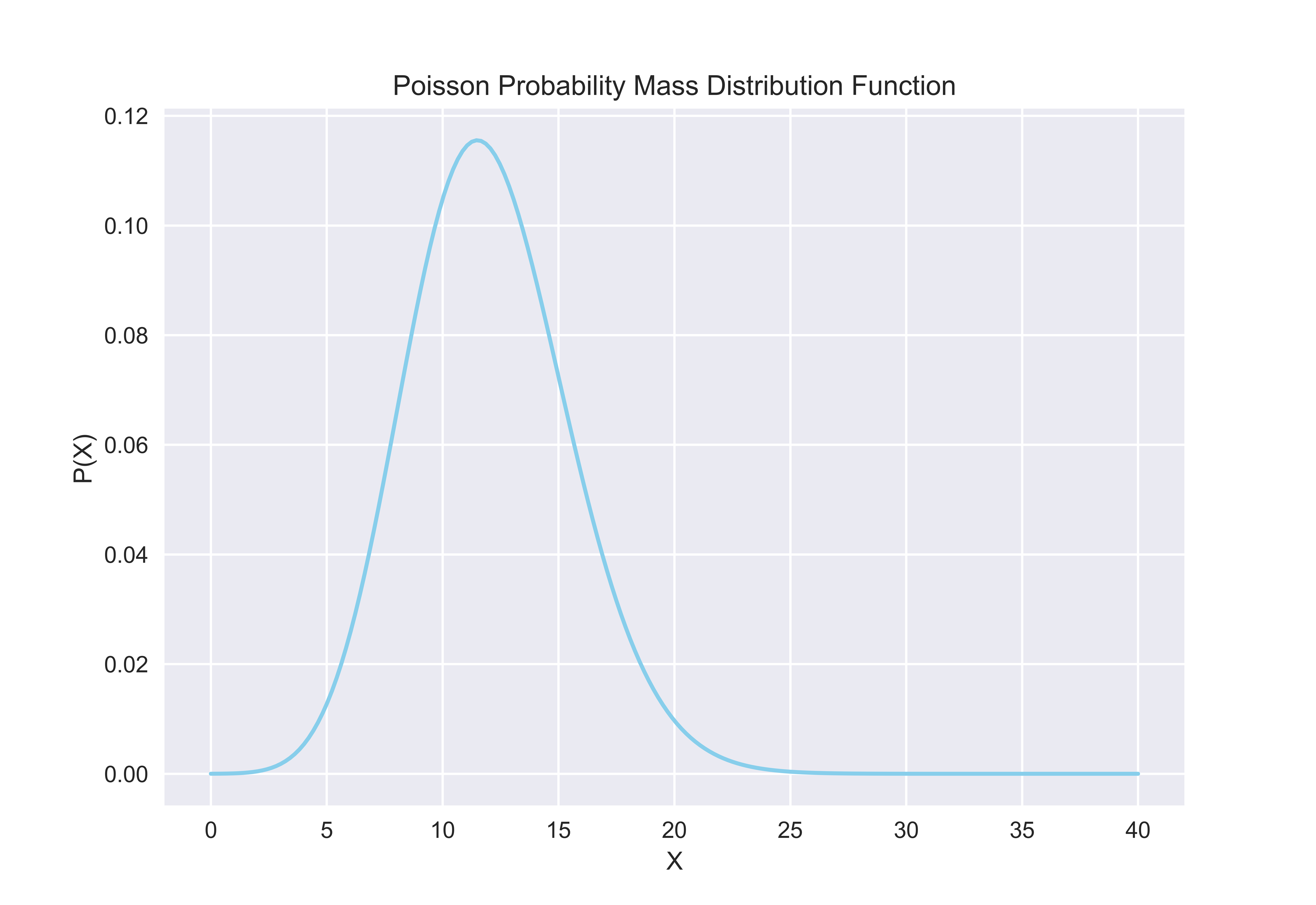
As expected, the graph peaks at \(x = 12\). At a glance, this distribution resembles the binomial distribution we looked at earlier, and indeed that is no coincidence: the Poisson distribution is essentially a special case of binomial distributions whereby the number of trials is literally pushed to the limit. As stated earlier, the binomial distribution can be considered as a very rough approximation of the Poisson distribution, and the accuracy of approximation would be expected to increase as \(n\) increases.
So let me ask the question again: how lucky was I yesterday? The probability distribution function of the Poisson distribution tells us that \(P(X = 5)\) can be calculated through the following equation:
\[P(X = 5) = e^{-12} \frac{12^5}{5!} = 6.14421 \cdot 10^{-6} \cdot \frac{248832}{120} \approx 0.013\]The result given by the Poisson distribution is somewhat larger than that derived from the binomial distribution, which was \(0.0071\). This discrepancy notwithstanding, the fact that I had a very lucky day yesterday does not change: I would have days like these once every 100 days, and those days surely don’t come often.
But to really calculate how lucky I get for the next 18 months of my life in the military, we need to do a bit more: we need to also take into account the fact that receiving lesser than 5 calls on a shift also constitutes a lucky day. In other words, we need to calculate \(\sum_{n=0}^5 P(X = n)\), as shown below:
\[\sum_{n=0}^5 P(X = n) = P(X = 0) + P(X = 1) + \dots + P(X = 5) = 0.02034\]This calculation can be done rather straightforwardly by plugging in numbers into the Poisson distribution function as demonstrated above. Of course, this is not the most elegant way to solve the problem. We could, for instance, tweak the Poisson distribution function and perform integration. The following is a code block that produces a visualization of what this integral would look like on a graph.
import numpy as np
from scipy.special import gamma

x = np.linspace(0, 40, 200)
y = np.exp(-12) * 12**x / gamma(x)
section = np.arange(0, 5, 1/20.)

plt.style.use("seaborn")
plt.grid(True)
plt.plot(x, y, 'skyblue')
plt.fill_between(section, np.exp(-12) * 12**section / gamma(section), color='skyblue')
plt.xlabel('X')
plt.ylabel('P(X)')
plt.title('Poisson Probability Mass Function')
plt.show()
Here is the figure produced by executing the code block above.

You might notice from the code block that the integrand is not quite the Poisson distribution—instead of a factorial, we have an unfamiliar face, the gamma(x) function. Why was this modification necessary? Recall that integrations can only be performed over smooth and continuous functions, hence the classic example of the absolute value as a non-integrable function. Factorials, unfortunately, also fall into this category of non-integrable functions, because the factorial operation is only defined for integers, not all real numbers. To remedy this deficiency of the factorial, we resort to the gamma function, which is essentially a continuous version of the factorial. Mathematically speaking, the gamma function satisfies the recursive definition of the factorial:
Using the gamma distribution function, we can then calculate the area of the shaded region on the figure above. Although I do not present the full calculation process here, the value is approximately equal to that we obtained above, \(0.02034\). So to answer the title of this post: about 2 in every 100 days, I will have a chill shift where I get lesser than five calls in eight hours. But all of this aside, I should make it abundantly clear in this concluding section that I like my job, and that I love answering calls on the phone. I can assure you that no sarcasm is involved.
If you insist on calculating this integral by hand, I leave that for a mental exercise for the keen reader. Or even better, you can tune back into this blog a few days later to check out my post on the gamma function, where we explore the world of distributions beyond the binomial and the Poisson.