Attention is All You Need
Today, we are finally going to take a look at transformers, the mother of most, if not all current state-of-the-art NLP models. Back in the day, RNNs used to be king. The classic setup for NLP tasks was to use a bidirectional LSTM with word embeddings such as word2vec or GloVe. Now, the world has changed, and transformer models like BERT, GPT, and T5 have now become the new SOTA.
Before we begin, I highly recommend that you check out the following resources:
- The Illustrated Transformer
- Illustrated Guide to Transformers Neural Network
- Attention and Transformer Networks
These resources were of enormous help for me in gaining a solid conceptual understanding of this topic. For implementation details, I referred to
And of course, it is my hope that this post also turns out to be helpful for those trying to break into the world of transformers. Let’s get started!
Introduction
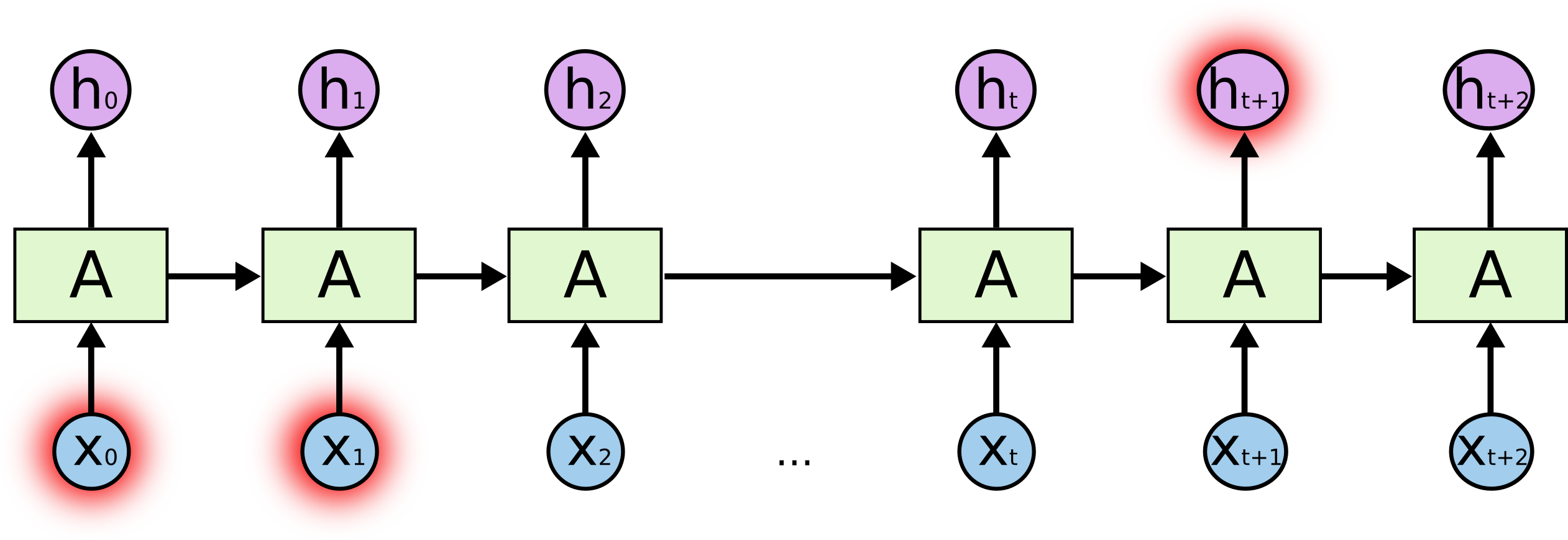
While LSTMs and other RNNs are effective at solving NLP tasks, they are only effective to a degree: due to the sequential nature with which data is processed, RNNs cannot handle long-range dependencies very well. This means that, when sentences get long, some data might be lost. This is an inherent limitation of RNNs, as they rely on hidden states that are passed throughout the unrolling sequence to store information about the input data. When it is unrolled for too many time steps, the hidden state can no longer accurately capture information from earlier on in the sequence. Below is an illustration taken from Chris Olah’s blog.
Transformers, unlike RNNs, are not recursive by nature. Instead, transformer models are able to digest sequential input data all at once in parallel. Therefore, they do not suffer from the long-range dependency problem. They are also generally quicker to train than LSTM networks, although this statement is somewhat undercut by the fact that recent transformer SOTA models are extremely massive to the extent that no individual developer can train them on a personal GPU from scratch. However, the massiveness of a network is not an inherent characteristic of the transformer architecture; it is better understood as a general trend in the bleeding-edge research community.
At a very high level, the transformer architecture is composed of two parts: an encoder and a decoder. Below is an illustration taken from the original paper that started it all, Attention is All You Need.

As can be seen, the transformer is definitely not the simplest of all models. However, upon closer examination, you might also realize that many of the components of the model are repeated and reused throughout the model. Specifically, we see that one sub-component of the encoder block is a multi-head attention layer with a residual connection and layer normalization. This unit can also be found in the decoder block, with the minor caveat that the decoder uses masked multi-head attention. The point-wise feed forward structure exists in both the encoder and decoder. Even the way input data is treated seems identical: both the encoder and decoder use an element-wise addition of the input and positional embeddings.
The objective here will simply be to implement the transformer architecture and gain a better understanding of how it works. We could of course train this model, but that is less the focus of this blog post, since the goal is to really see how the transformer works under the hood. Of course, one could use the HuggingFace transformers library without really understanding how transformers work, but it’s always nice to have some knowledge of what’s actually happening under the hood of a transformer model. For now, let’s focus on the implementation details.
With these details in mind, let’s try implementing this beast.
Transformer Encoder
As always, we will be using PyTorch for this tutorial.
import torch
from torch import nn
import torch.nn.functional as F
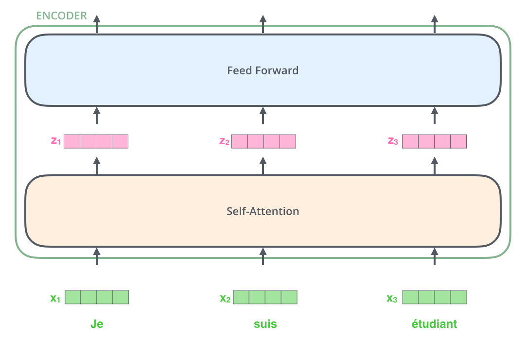
Recall the the transformer architecture borrows the encoder-decoder sturcture commonly found in seq2seq or autoencoder models. Let’s start with the encoder. Zooming into the encoder block, we see a structure as shown below. The image was taken from Jay Alammar’s blog post.
![]()
Positional Embedding
The first step of this process is creating appropriate embeddings for the transformer. Unlike RNNs, transformers processes input tokens in parallel. Because of this, we need to provide the model with some sense of order and time; otherwise, it would consider the tokens as simply a bag of words or some random permutation. Therefore, we need to create what’re called positional embeddings.
![]()
As you can see, the embeddings are added with positional embeddings that encode information about the absolute position of the token in the sequence. This is how the transformer can learn temporal or sequential information that would have otherwise been lost. It is also worth noting that the dimensions of the positional embedding and the semantic embedding must match in order for the two vectors to be added.
Self-Attention
Once we create a combined embedding using positional encoding, we then pass these embeddings through an encoder block. The encoder is nothing but a stack of these encoder blocks that are repeated throughout the architecture, which is why it is very important to have a solid understanding of the inner workings of a single encoder block.
The first core piece of the encoder block is the multi-head self-attention layer. This component is arguably the core contribution of the authors of Attention is All You Need.
To understand multi-head self-attention, let’s review what attention is in the first place. Recall that attention is a mechanism used to efficiently transfer information from the encoder to the decoder. When the decoder decodes some input data, it refers back to the hidden states produced by the seq2seq encoder to learn which encoding time step is most relevant to the current decoding process. Visually, this process can be illustrated as follows:
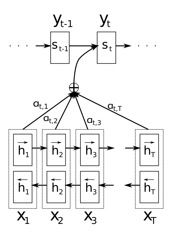
In the diagram above, $h_n$ refers to the hidden states produced by the encoder RNN at time step $n$; the decoder at the $t$-th time step then views all the encoder hidden states and uses some attention mechanism to figure out which hidden state is the most relevant. It then creates a weighted average vector using attention weights $a_n$, then uses that averaged vector in the decoding computation process.
Multi-head self-attention is similar to this process, but with a major caveat: instead of having the decoder learning which part of the encoder output to attend to, we train the encoder to learn which part of its own input sequence to attend to, hence the term “self-attention.” This can be somewhat confusing on paper, so let’s concrete with an example.
Say we have a sentence, “The animal didn’t cross the street because it was too tired.”

Using self-attention, the model basically uses the input embeddings in the sequence to compare it with the sequence itself, as seen above. At first glance, you might think this makes no sense. After all, it’s not like there is an encoder and decoder; this self-attention layer exists inside the encoder and has nothing to do with the decoder of the transformer. However, you might also see from the illustration above that self-attention can make a lot of sense when, say, we want to teach the model to understand pronouns like “it.” In the example above, the model learns to attend to the word “animal” while looking at the token “it.” This is because, grammatically, “animal” is what “it” is referring to. In short, through self-attention, the model learns these patterns within the data itself. This is also one way through which transformers can overcome long range dependencies.
The explanation above is good intuition to have, but we’ve not gotten into the details of what how it works, so let’s take a deeper look. In self-attention, we have three core components:
- Key
- Value
- Query
Consider a database lookup operation. In SQL, you might look for a specific entry by doing something like
SELECT col1, col2
FROM table_name
WHERE condition;
For django fans like me, you might have also seen something like
Table.objects.get(condition) # could also use .filter().first()
Regardless of the platform or framework, the underlying idea behind database lookups is simple: you retrieve some values in the database whose keys correspond to or satisfy the condition specified in the query.
With this context in mind, let’s go back to the example of
“The animal didn’t cross the street because it was too tired.”
When the model looks at the word “it,” it will calculate self-attention over all words in the sequence, including itself. However, we expect a trained model to especially attend to “animal,” as that is what the pronoun is actually referring to in the sentence. In other words, given the query “it,” we expect the model attribute high attention to the key “animal,” and thus use the embedding of “animal” a lot when calculating that weighted average attention vector we talked about in the context of general attention. In self-attention terms, we refer to this weighted average vector as context embeddings.
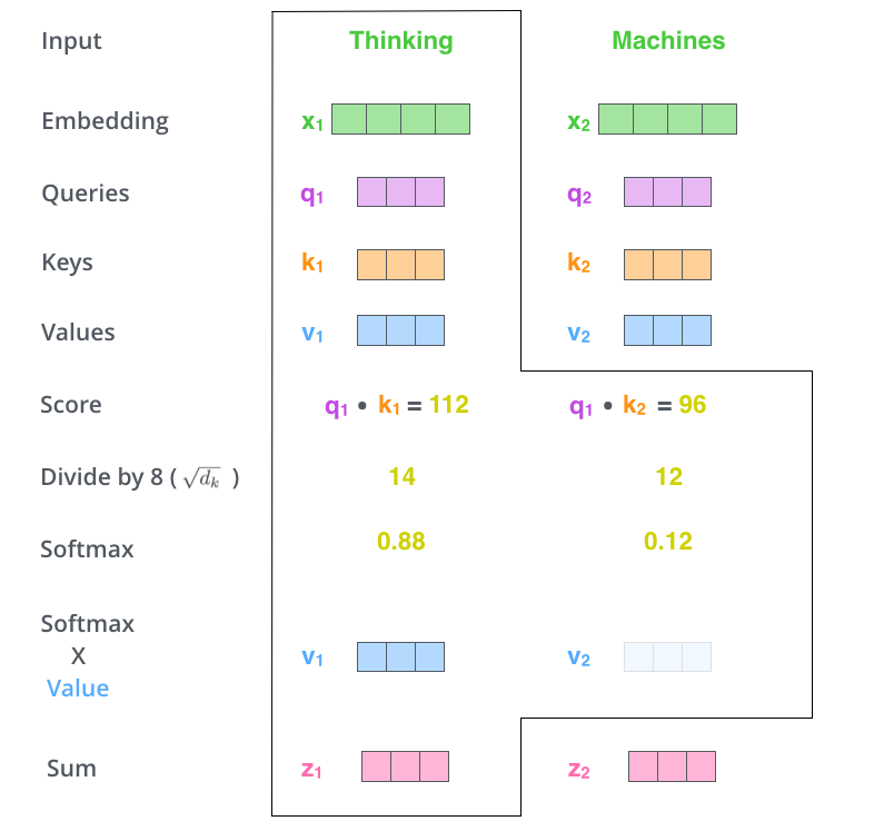
Above is another illustration from Jay Alammar’s blog that wonderfully demonstrates how self-attention can be used to create context embeddings. In the example here, we’re looking at a phrase of two words, “thinking machines.” At the first encoding time step, the encoder will look at “thinking” and calculate attention across both “thinking” and “machines.” In other words, we use the query vector that corresponds to “thinking” and compare it with keys for “thinking” and “machines.” We calculate the score, sometimes referred to as energy, by taking a dot product between the queries and keys. The intuition is that the larger this dot product, the more related the two tokens are. We then take the softmax of the energy vector to then create a weighted values vector. We refer to these vectors as context embeddings since they encode information regarding the context surrounding that token via self-attention. Put more formally, self-attention can be written as follows:
\[\text{Attention}(Q, K, V) = \text{softmax}\left(\frac{Q K^\top}{\sqrt{d_k}} \right) V\]The original paper divides self-attention by the dimensions of the hidden embedding vector to stabilize gradients and remove variance, but this is details beyond the scope of this post. For now, it suffices to see that self-attention is a dot product that can easily be calculated in a vectorized fashion via matrix multiplication.
Multi-Head Attention
So far, we’ve looked at how self-attention works. Now, it’s time to understand where the multi-head part comes in.
The short answer is that multi-head self-attention is nothing but a parallel repetition of self-attention. In other words, instead of only having one key-value pair for each token, we have multiple. This is best illustrated by the visualization on the original paper.

We see that there is the familiar scaled dot-product attention we’ve discussed above, but with many layers. Specifically, there are $h$ scaled dot-products we see in the diagram above. This is all there is to the multi portion of multi-head self-attention.
The more important question is why we might one multi-head attention in the first place. The reason lies in nothing but the same reason why we might want to have more neurons in a feature. By having multiple key-value pairs, we are able to extract more features from the token sequence. More intuitively, the multi-headedness of the self-attention mechanism can also provide a more reliable guarantee that the self-attention layer not only learns to attend to the current token, but other related tokens that could be near or far away in the sequence.
Now that we have an overall understanding of how positional embedding, self-attention, and multi-head self-attention works, let’s get our hands dirty with some PyTorch code.
Implementation
Let’s first start by considering the overall shell of an encoder. As seen in the diagrams above, the transformer encoder largely requires only two components:
- Positional embedding
- Encoder layers
The encoder structure, presented below, assumes that we have already implemented the encoder layer. The main point of the encoder is to observe how the final input embeddings are created by adding positional and token embeddings.
It should be noted that positional encoding was actually implemented quite differently in the original paper. Specifically, the authors use trigonometric functions of different periods to make positional embeddings constant vectors. Consider, for instance, this example from Harvard NLP’s annotated transformer:
![]()
In this example, there are a total of 4 trigonometric functions, so we could consider it a four-dimensional positional encoding generation technique. The $x$-axis represents the absolute position of the token in the input sequence. Then, we can read the $y$-values of each graph to obtain a vector. Note that no vector is identical despite the cyclic nature of trigonometric graphs, at least up to the point that is plotted in the graph. If we add more functions, we would expect the longer dimensional positional embedding to be unique for each position.
While this approach certainly works, the more mainstream technique now is to make positional embeddings a trainable parameter. Namely, we treat positional embeddings just like any other embedding layer. The only difference is that this positional embedding layer simply takes as input an integer sequence from 0 up to the sequence length.
class Encoder(nn.Module):
    def __init__(
        self,
        vocab_size,
        embed_dim,
        max_len,
        num_layers,
        num_heads,
        ff_hid_dim,
        dropout=0.5,
    ):
        super().__init__()
        self.tok_embed = nn.Embedding(vocab_size, embed_dim)
        self.pos_embed = nn.Embedding(max_len, embed_dim)
        self.layers = nn.ModuleList(
            [
                EncoderLayer(embed_dim, num_heads, ff_hid_dim, dropout)
                for _ in range(num_layers)
            ]
        )
        self.dropout = nn.Dropout(dropout)

    def forward(self, src, src_mask):
        batch_size = src.size(0)
        seq_len = src.size(1)
        device = next(self.parameters()).device
        pos = (
            torch.arange(0, seq_len)
            .unsqueeze(0)
            .repeat(batch_size, 1)
            .to(device)
        )
        src = self.dropout(self.pos_embed(pos) + self.tok_embed(src))
        for layer in self.layers:
            src = layer(src, src_mask)
        return src
The part the deserves the most attention is how positional embeddings are dynamically created in the forward method of the model. With some tensor dimensions manipulation, we add the positional and token embeddings to create the final embedding to be fed into the encoder layers.
The encoder layer itself is also pretty simple. Here, we again assume that we have already implemented the multi-head self-attention layer as well as the point-wise feed forward network that follows.
So really, all we need is to put the two pieces together. As a minor implementation detail, we add dropout to ensure that the model does not overfit. We also add layer normalization as was stated in the original paper. Layer normalization is similar to batch normalization, but there are major differences. Roughly speaking, batch normalization keeps a weighted exponential average across each dimension across batches, whereas layer normalization simply normalizes each individual sample.

While I tried to find good explanations and illustrations, I found most of them somewhat confusing. The best way to really see the difference is to test it out some dummy data.
layer_norm = nn.LayerNorm(2)
batch_norm = nn.BatchNorm1d(2)
data = torch.arange(0, 10).reshape(5, 2).to(torch.float32)
In the case of layer normalization, we see that each individual sample was independently normalized.
layer_norm(data)
tensor([[-1.0000,  1.0000],
        [-1.0000,  1.0000],
        [-1.0000,  1.0000],
        [-1.0000,  1.0000],
        [-1.0000,  1.0000]], grad_fn=<NativeLayerNormBackward>)
In the case of batch normalization, the samples were normalized across the batch dimension.
batch_norm(data)
tensor([[-1.4142, -1.4142],
        [-0.7071, -0.7071],
        [ 0.0000,  0.0000],
        [ 0.7071,  0.7071],
        [ 1.4142,  1.4142]], grad_fn=<NativeBatchNormBackward>)
This necessarily means that the sum of the output across batch dimension will have zero mean and variance.
batch_norm(data).sum(dim=0)
tensor([0., 0.], grad_fn=<SumBackward1>)
Empirically, researchers have found layer normalization to be effective, and so we follow the original paper in our implementation. Let’s see how we can build a basic encoder layer using layer normalization and multi-head self-attention.
class EncoderLayer(nn.Module):
    def __init__(
        self, embed_dim, num_heads, ff_hid_dim, dropout
    ):
        super().__init__()
        self.ff_ln = nn.LayerNorm(embed_dim)
        self.attention_ln = nn.LayerNorm(embed_dim)
        self.ff = FeedForward(embed_dim, ff_hid_dim, dropout)
        self.attention = MultiHeadAttention(embed_dim, num_heads)
        self.dropout = nn.Dropout(dropout)

    def forward(self, src, src_mask):
        attention_out = self.attention(src, src, src, src_mask)
        attetion_ln_out = self.dropout(self.attention_ln(src + attention_out))
        ff_out = self.ff(attetion_ln_out)
        ff_ln_out = self.dropout(self.ff_ln(attetion_ln_out + ff_out))
        return ff_ln_out
You might have realized that the attention layer takes as input three components: key, value, query, and a mysterious mask. The mask is used to prevent the model from seeing some tokens in the input sequence. Since we are dealing with batched inputs, we can easily see how there might be some extraneous padding tokens that we don’t want the model to necessarily pay attention to. We hide these tokens from the multi-head attention layer by passing in a mask, so that the model can pay attention to only parts that matter. We will get more specific on masks in the decoder layer.
Finally, we come to the heart of the transformer model, the multi-head self-attention layer. Initially, I thought about creating a key, value, and query matrix for each head and using batch matrix multiplication. However, after looking at a few implementations, I realized that one could achieve a similar effect by considering different heads all at once in a single matrix. In other words, we simply create a single matrix for key, value, and queries, assuming that the single giant matrix is a concatenation of the different heads. Then, it must be that
\[D_\text{hidden} = N_\text{head} \cdot D_\text{head}\]where $D$ denotes the dimension and $N$ denotes count. With this thought process in mind, and with some convoluted matrix dimension operations, we can come up with the following implementation. For sake of clarity, I’ve annotated dimensions of each variable.
class MultiHeadAttention(nn.Module):
    def __init__(self, hid_dim, num_heads):
        super().__init__()

        assert hid_dim % num_heads == 0, "`hidden_dim` must be a multiple of `num_heads`"

        self.hid_dim = hid_dim
        self.num_heads = num_heads
        self.head_dim = hid_dim // num_heads

        self.fc_v = nn.Linear(hid_dim, hid_dim, bias=False)
        self.fc_k = nn.Linear(hid_dim, hid_dim, bias=False)
        self.fc_q = nn.Linear(hid_dim, hid_dim, bias=False)
        self.fc = nn.Linear(hid_dim, hid_dim)

    def forward(self, value, key, query, mask=None):
        # keys.shape = [batch_size, seq_len, embed_dim]
        batch_size = query.size(0)

        V = self.fc_v(value)
        K = self.fc_k(key)
        Q = self.fc_q(query)
        # shape = [batch_size, seq_len, hid_dim]

        V = V.reshape(batch_size, -1, self.num_heads, self.head_dim).permute(0, 2, 1, 3)
        K_t = K.reshape(batch_size, -1, self.num_heads, self.head_dim).permute(0, 2, 3, 1)
        Q = Q.reshape(batch_size, -1, self.num_heads, self.head_dim).permute(0, 2, 1, 3)
        # V.shape = [batch_size, num_heads, value_len, head_dim]
        # K_t.shape = [batch_size, num_heads, head_dim, key_len]

        energy = torch.matmul(Q, K_t) / (self.hid_dim ** 1/2)
        # energy.shape = [batch_size, num_heads, query_len, key_len]

        if mask is not None:
            energy = energy.masked_fill(mask == 0, float("-inf"))

        attention = F.softmax(energy, dim=-1)
        weighted = torch.matmul(attention, V)
        # weighted.shape = [batch_size, num_heads, seq_len, head_dim]
        weighted = weighted.permute(0, 2, 1, 3)
        # weighted.shape = [batch_size, seq_len, num_heads, head_dim]
        weighted = weighted.reshape(batch_size, -1, self.hid_dim)
        # weighted.shape = [batch_size, seq_len, hid_dim]
        out = self.fc(weighted)
        # out.shape = [batch_size, seq_len, hid_dim]
        return out
Despite the somewhat complicated matrix dimension permutation logic, the key takeaway is the fact that we compute the dot product between the key and query to create a weighted average of the values corresponding to each key, which we refer to as the contextual embedding. The raw value calculated by the dot product is stored in the energy matrix.
The masking that happens in the middle of the forward function lends some insight into how masking works and what it is intended to achieve. A simple intuition is that negative infinity, when passed into a softmax function, outputs zero. Therefore, we use the mask as reference to set some elements of energy equal to negative infinity before passing it through the softmax function.
Next up is the point-wise feed forward network. This is the layer that follows the multi-head self-attention. The idea is that we expand the dimensions of the network through a hidden state and apply an additional layer of non-linearity to add representational complexity to the model. But for the most part, nothing interesting happens here.
class FeedForward(nn.Module):
    def __init__(self, embed_dim, hid_dim, dropout):
        super(FeedForward, self).__init__()
        self.fc1 = nn.Linear(embed_dim, hid_dim)
        self.fc2 = nn.Linear(hid_dim, embed_dim)
        self.dropout = nn.Dropout(dropout)

    def forward(self, x):
        return self.fc2(F.relu(self.dropout(self.fc1(x))))
In the paper, the authors use GELU, or Gaussian Error Linear Units. For the sake of simplicity, however, I decided to use the more familiar ReLU. For a more detailed dive into what GELU is, I recommend that you check out this stack exchange post.
Now, we have finally implemented all components of the encoder! This might have felt a little confusing due to the top-down approach we took, starting from the entire encoder model from the ground-up then narrowing down into its sub-components like the encoder layer, multi-head self-attention, and the point-wise feed forward network. Nonetheless, we are more than half way done in our journey. Now is time to turn our attention (no pun intended) to the other half of the model, the decoder.
Transformer Decoder
The good news is that we have already built most of what we need for the decoder. Specifically, we have already implemented duplicated components, such as the multi-head self-attention and the feed forward network. All there is left is to put the pieces together, and of course some decoder-specific work that has to be done. And largely due to this fact, I’d like to preface this section with the statement that portion will be a lot shorter than the previous one on the encoder architecture.
Let’s start with the birds-eye view of the decoder.
class Decoder(nn.Module):
    def __init__(
        self,
        vocab_size,
        embed_dim,
        max_len,
        num_layers,
        num_heads,
        ff_hid_dim,
        dropout=0.5,
    ):
        super().__init__()
        self.tok_embed = nn.Embedding(vocab_size, embed_dim)
        self.pos_embed = nn.Embedding(max_len, embed_dim)
        self.layers = nn.ModuleList(
            [
                DecoderLayer(embed_dim, num_heads, ff_hid_dim, dropout)
                for _ in range(num_layers)
            ]
        )
        self.dropout = nn.Dropout(dropout)
        self.fc = nn.Linear(embed_dim, vocab_size)

    def forward(self, trg, trg_mask, enc_src, src_mask):
        batch_size = trg.size(0)
        seq_len = trg.size(1)
        device = next(model.parameters()).device
        pos = (
            torch.arange(0, seq_len)
            .unsqueeze(0)
            .repeat(batch_size, 1)
            .to(device)
        )
        trg = self.dropout(self.pos_embed(pos) + self.tok_embed(trg))
        for layer in self.layers:
            trg = layer(trg, trg_mask, enc_src, src_mask)
        out = self.fc(trg)
        return out
Much like the encoder, the decoder also makes use of positional embedding. The mechanism through which we achieve this is also identical: we use an additional layer of embedding dedicated to encoding sequential information and simply concatenate it with the token embeddings. The only difference is that, quite obviously, we now use a stack of decoder layers instead of encoder layers.
Decoder Layer
Next, we implement the decoder layer. The decoder layer is where we start to see some differences between the encoder and decoder. Namely, the decoder block contains two attention blocks: one for the processing multi-head self-attention using data from the output generated sequence, and another for computing attention between the encoder and decoder outputs. Note that the second attention block can be understood as the traditional seq2seq-style attention between the encoder and decoder we discussed earlier.
For the sake of completeness, below is the overall structure of the transformer network.
![]()
As can be seen, each decoder layer accepts contextual embeddings created by the encoder as input. This means that the forward method of the decoder will take encoder outputs as a parameter.
class DecoderLayer(nn.Module):
    def __init__(self, embed_dim, num_heads, ff_hid_dim, dropout):
        super().__init__()
        self.ff_ln = nn.LayerNorm(embed_dim)
        self.dec_attn_ln = nn.LayerNorm(embed_dim)
        self.enc_attn_ln = nn.LayerNorm(embed_dim)
        self.ff = FeedForward(embed_dim, ff_hid_dim, dropout)
        self.dec_attn = MultiHeadAttention(embed_dim, num_heads)
        self.enc_attn = MultiHeadAttention(embed_dim, num_heads)
        self.dropout = nn.Dropout(dropout)

    def forward(self, trg, trg_mask, enc_src, src_mask):
        dec_attn_out = self.dropout(self.dec_attn(trg, trg, trg, trg_mask))
        dec_attn_ln_out = self.dec_attn_ln(trg + dec_attn_out)
        enc_attn_out = self.dropout(
            self.enc_attn(enc_src, enc_src, dec_attn_ln_out, src_mask)
        )
        enc_attn_ln_out = self.enc_attn_ln(dec_attn_ln_out + enc_attn_out)
        ff_out = self.dropout(self.ff(enc_attn_ln_out))
        ff_ln_out = self.ff_ln(ff_out + enc_attn_ln_out)
        return ff_ln_out
We see that there are two attention layers: a multi-head self-attention layer similar to the one we’ve seen in the encoder, and the more traditional encoder-decoder attention we’ve seen in seq2seq models. After the two attention layers, we again have a point-wise feed forward network where we increase the number of hidden units, apply a non-linearity, then revert back to the original embedding dimension.
There some pieces of the decoder layer that should be highlighted. First, the decoder multi-head self-attention obviously takes the target input as keys, values, and queries. WE also use the target data mask, denoted as trg_mask. We will discuss what this is more specifically below, but basically it is a mask we use to prevent the decoder from looking ahead in the decoding sequence. In the next attention layer, the encoder-decoder attention, is slightly different. Namely, we use the decoder output as queries, and use encoder outputs as keys and values. The source mask is used here, since obviously we don’t want source mask tokens to interfere in this attention computation process.
Transformer
Now, we have all the pieces we need: all we need to do is to put the pieces together into a single model class, aptly dubbed the Transformer in the snippet below.
class Transformer(nn.Module):
    def __init__(
        self,
        src_vocab_size,
        trg_vocab_size,
        src_pad_idx,
        trg_pad_idx,
        embed_dim=512,
        max_len=100,
        num_layers=6,
        num_heads=8,
        ff_hid_dim=2048,
        dropout=0.5,

    ):
        super().__init__()
        self.encoder = Encoder(
            src_vocab_size,
            embed_dim,
            max_len,
            num_layers,
            num_heads,
            ff_hid_dim,
            dropout,
        )
        self.decoder = Decoder(
            trg_vocab_size,
            embed_dim,
            max_len,
            num_layers,
            num_heads,
            ff_hid_dim,
            dropout,
        )
        self.src_pad_idx = src_pad_idx
        self.trg_pad_idx = trg_pad_idx

    def make_src_mask(self, src):
        # src.shape = [batch_size, src_len]
        src_mask = (src != self.src_pad_idx).unsqueeze(1).unsqueeze(2)
        # src.shape = [batch_size, 1, 1, src_len]
        return src_mask

    def make_trg_mask(self, trg):
        batch_size = trg.size(0)
        seq_len = trg.size(1)
        pad_mask = (trg != self.trg_pad_idx).unsqueeze(1).unsqueeze(2)
        seq_mask = torch.tril(torch.ones(seq_len, seq_len))
        trg_mask = pad_mask * seq_mask
        return trg_mask

    def forward(self, src, trg):
        device = next(model.parameters()).device
        src_mask = self.make_src_mask(src).to(device)
        trg_mask = self.make_trg_mask(trg).to(device)
        enc_src = self.encoder(src, src_mask)
        decoder_out = self.decoder(trg, trg_mask, enc_src, src_mask)
        return decoder_out
Most of what is shown above is unsurprising. We simply pass the source into the encoder, then pass the encoded output to the decoder. The only part that requires some highlighting is the masking portion of the code. Let’s take a deeper look at what the encoder and decoder masks are.
First, let’s think about what mask the encoder should be given. To make things more concrete, let’s consider the following dummy example. We use 0 as padding indices, and have a vocabulary size of 10 for both source and target languages.
src_pad_idx = 0
trg_pad_idx = 0
src_vocab_size = 10
trg_vocab_size = 10
device = torch.device("cuda" if torch.cuda.is_available() else "cpu")
src = torch.tensor(
    [[1, 5, 6, 4, 3, 9, 5, 2, 0], [1, 8, 7, 3, 4, 5, 6, 7, 2]]
).to(device)
trg = torch.tensor([[1, 7, 4, 3, 5, 0, 0, 0], [1, 5, 6, 2, 4, 7, 6, 2]]).to(
    device
)
The motivating idea is that we don’t want the model to be calculating self-attention for any padding tokens since they are supposed to carry no meaning. Therefore, we want to apply a mask so that the model doesn’t see the padding tokens.
We can easily create a mask by using a boolean operator, namely checking whether each element is or is not equal to the masking token.
src_mask = (src != src_pad_idx).unsqueeze(1).unsqueeze(2)
src_mask
tensor([[[[ True,  True,  True,  True,  True,  True,  True,  True, False]]],
        [[[ True,  True,  True,  True,  True,  True,  True,  True,  True]]]])
You might be wondering why it is necessary to squeeze the mask twice to create extraneous dimensions. If you recall where the masks are applied in the self-attention layer, you will see this:
# energy.shape = [batch_size, num_heads, query_len, key_len]
energy = energy.masked_fill(mask == 0, float("-inf"))
Since the shape of the original input is
src.shape
torch.Size([2, 9])
we want to create additional dimensions along the heads and query length dimension.
src_mask.shape
torch.Size([2, 1, 1, 9])
The most important takeaway here is that the mask hides the keys. If you look carefully at the dimensions of the energy tensor and the mask, you will see that the mask coincides with the energy in the last key dimension. In other words, the mask effectively prevents the model from seeing certain keys, namely those whose token corresponds to the padding token. As we see in the code above, we can easily check for padding tokens by using a simple equality.
The story is not too much different for the decoder, but there are some more interesting details to be hashed out. An important detail for the decoder is that the decoder should not see the tokens beyond its current time step. If not, the model would learn to cheat by basically just looking at the rest of the target sequence and regurgitating its content. For example, if we want the model to decode out a translation, “I love you,” at the point in which the model is on “love,” it should not have access to “you”; the goal is to make the model to predict “you.” Therefore, we need to apply masking on not only the keys, but also the queries themselves.
To make this more concrete, let’s create the model and see what target mask gets created.
model = Transformer(
    src_vocab_size, trg_vocab_size, src_pad_idx, trg_pad_idx
).to(device)
We want the model to predict the end-of-sentence token. Therefore, given the following full target sequence,
trg = [<sos>, y1, y2, ..., yt, <eos>]
we will only be passing in up until the second to last token.
trg = [<sos>, y1, y2, ..., yt]
The model should the predict the full sequence.
trg_pred = [y1, y2, ..., yt, <eos>]
Therefore, we would only pass in trg[:, :-1], indexing until the second last token in the batch.
Let’s take a look at what the target mask looks like.
trg_mask = model.make_trg_mask(trg[:, :-1])
trg_mask
tensor([[[[1., 0., 0., 0., 0., 0., 0.],
          [1., 1., 0., 0., 0., 0., 0.],
          [1., 1., 1., 0., 0., 0., 0.],
          [1., 1., 1., 1., 0., 0., 0.],
          [1., 1., 1., 1., 1., 0., 0.],
          [1., 1., 1., 1., 1., 0., 0.],
          [1., 1., 1., 1., 1., 0., 0.]]],

        [[[1., 0., 0., 0., 0., 0., 0.],
          [1., 1., 0., 0., 0., 0., 0.],
          [1., 1., 1., 0., 0., 0., 0.],
          [1., 1., 1., 1., 0., 0., 0.],
          [1., 1., 1., 1., 1., 0., 0.],
          [1., 1., 1., 1., 1., 1., 0.],
          [1., 1., 1., 1., 1., 1., 1.]]]])
We see that the target mask is a triangular matrix. With some thinking, it is not difficult to convince ourselves that this is indeed the shape we want. Recall the self-attention, which manifests in the form of energy, is a matrix between the queries and keys to the layer. We mask the keys at different time steps so that the model cannot look ahead of the decoding sequence. Also, just like the encoder, we make sure that we mask out the padding tokens. You will see, for instance, that the first matrix in the mask above is not strictly triangular since the last few rows are masked due to padding.
Note that the energy matrix is of shape [batch_size, num_heads, query_len, key_len]. The idea is that the keys should only have access to preceding tokens in the query. This is clearly different from what we saw in the encoder attention: the encoder can see everything, so of course, the keys can have access to all the queries. This is why the target mask has a shape that is different from that of the source mask.
trg_mask.shape
torch.Size([2, 1, 7, 7])
Now, we can finally run the sanity check to see that the model can run a proper forward pass without any issues. This is a very cheap yet easy way to test that an implementation works.
out = model(src, trg[:, :-1])
out.shape
torch.Size([2, 7, 10])
And it does! The prediction will of course be meaningless garbage since the model has not been trained, but at least we know that the model has output 10 predictions for each example, which is equal to the number of the size of the vocabulary.
Conclusion
Today, we’ve taken a pretty thorough look into how transformers work. This is one of the most personally rewarding posts I’ve written, largely because I’ve meant to understand transformers for a while now. I’ve used BERT and have seen a lot of videos on the sheer magic of GPT-2 and GPT-3, yet never had the chance to really dive deep into how these work. Granted, this post was not about the aforementioned transformer models, but about the more general, vanilla transformer model that was first announced. However, understanding the clockwork of transformers is pivotal to realizing how these other more complicated, recent models work in practice. For instance, BERT is really just a stack of encoders, and GPT is a stack of decoders. I hope to explore these models in more detail in the posts to come.
I hope you’ve enjoyed reading this post. Catch you up in the next one!