Attention Mechanism
Attention took the NLP community by storm a few years ago when it was first announced. I’ve personally heard about attention many times, but never had the chance to fully dive into what it was. In this post, we will attempt to bake in a simple attention mechanism into a seq2seq model. This post builds on top of the seq2seq-related topics we have been exploring last month. Without further ado, let’s jump right in!
Concept
Let’s recall the improved seq2seq model we built in the last post. This diagram was taken from Ben Trevett’s repository on which this post is also based.
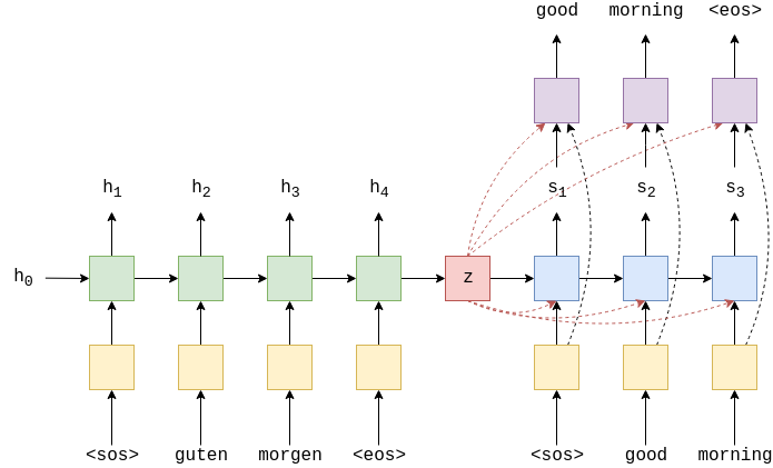
As you can see, we reduced the compression burden on the final $z$ output vector by allowing the decoder to have access to the output vector at all time steps of the decoding process. This is different from the vanilla seq2seq model, where the final encoding output is only available at the first time step and is diluted throughout the decoding process.
However, the fact that the encoding output should still contain all relevant information from the input remains unchanged. This could be a problem if, say, the input is an extremely long sequence. In that case, we cannot reasonably expect $z$ to be able to contain all information from the input without non-trivial loss. This is where attention comes to the rescue!
The most salient advantage of using attention is that, with attention, the decoder now has access to all the hidden states of the encoder. So instead of generating a highly compact, compressed version of the input via the encoder output $z$, instead the decoder can now “see” all the hidden states from the encoder and pay attention to the hidden states that matter most. Intuitively, this makes a lot of sense: in a machine translation setting, for example, the decoder should attend to “guten” when translating “good” and pay lesser attention to “morgen.” The end goal here is that the seq2seq model can learn some correspondence between some tokens and others in the input and output sequence; in other words, understand the syntactic difference between different languages.
Here is a quick visualization of the attention model we will be implementing today.
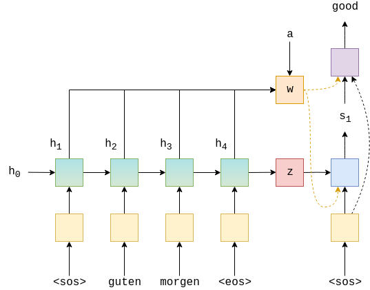
As you can see, every hidden state at each time step is used to calculate some new vector $w$, which is then passed in as input to both the decoder as well as the final output classifier. While the diagram only shows one time step, this process occurs at every decoding time step: a new vector is calculated using all the hidden states with attention, and passed in as input to the decoder at the specific time step.
You might be wondering how this mysterious new vector is created. The idea is actually pretty simple: $w$ is but an attention-weighted average of the hidden states. In other words,
\[w = \sum a_i h_i\]where $a_i$ represents the attention on the $i$th hidden state; $h_i$, the $i$th hidden state. Note that $a_i$ is a scalar, whereas as $h_i$ is a vector. The higher the value of $a_i$, the more attention the model is paying to the $i$th sequence in the encoding step.
Now that we’ve drawn a general picture of what the attention-based seq2seq model should look like, let’s start building this model!
Implementation
Below are the modules we will need for this tutorial.
import random
import time

import torch
import torchtext
from torch import nn
import torch.nn.functional as F
from torchtext.data import BucketIterator, Field
from torchtext.datasets import Multi30k
The setup process, using torchtext fields, is identical to the steps we’ve gone through in previous tutorials, so I’ll go through them very quickly.
SRC = Field(
    tokenize="spacy",
    tokenizer_language="de",
    init_token="<sos>",
    eos_token="<eos>",
    lower=True,
)

TRG = Field(
    tokenize="spacy",
    tokenizer_language="en",
    init_token="<sos>",
    eos_token="<eos>",
    lower=True,
)

train_data, validation_data, test_data = Multi30k.splits(
    root="data", exts=(".de", ".en"), fields=(SRC, TRG)
)

SRC.build_vocab(train_data, max_size=10000, min_freq=2)
TRG.build_vocab(train_data, max_size=10000, min_freq=2)
Next, we create iterators to load the dataset to be fed into our model. These iterators are effectively data loaders in PyTorch.
BATCH_SIZE = 128
device = torch.device('cuda' if torch.cuda.is_available() else 'cpu')

train_iterator, validation_iterator, test_iterator = BucketIterator.splits(
    (train_data, validation_data, test_data), batch_size=BATCH_SIZE, device=device
)
Below, we can see that all data have properly been batched. Notice that the length of each batch is different; of course, within each batch, all sentences have the same length. Otherwise, they wouldn’t be a batch in the first place. However, it is apparent from this design that one benefit of using torchtext for batching data is that there is no need to worry about zero padding each sentence to make their lengths uniform across all batches.
for i, batch in enumerate(train_iterator):
    print(batch.src.shape)
    if i == 5:
        break
torch.Size([37, 128])
torch.Size([28, 128])
torch.Size([28, 128])
torch.Size([37, 128])
torch.Size([28, 128])
torch.Size([27, 128])
Modeling
Now is the time for the fun part: modeling and implementing attention. Recall the fact that attention mechanisms originally arose in the context of sequence-to-sequence modeling. The underlying question is this: when some information is encoded via the encoder, then decoded by the decoder, can the decoder learn which part of the encoding to focus on while decoding? An easy real-life example of this would be machine translation. Given the input “I love you,” the Korean translation would be “나는 너를 사랑해,” or, translated word by word “I you love.” In this particular instance, the decoder has to know that there is some syntactic difference between Korean and English, and know which part of the original English sequence to focus on when producing a translation.
Encoder
Now that we have some idea of what attention is, let’s start coding the encoder.
class Encoder(nn.Module):
    def __init__(
        self,
        vocab_size,
        embed_dim,
        encoder_hidden_size,
        decoder_hidden_size,
        dropout
    ):
        super(Encoder, self).__init__()
        self.dropout = nn.Dropout(dropout)
        self.embed = nn.Embedding(vocab_size, embed_dim)
        self.gru = nn.GRU(embed_dim, encoder_hidden_size, bidirectional=True)
        self.fc = nn.Linear(encoder_hidden_size * 2, decoder_hidden_size)

    def forward(self, x):
        embedding = self.dropout(self.embed(x))
        outputs, hidden = self.gru(embedding)
        # outputs.shape == (seq_len, batch_size, 2 * encoder_hidden_size)
        # hidden.shape == (2, batch_size, encoder_hidden_size)
        concat_hidden = torch.cat((hidden[-1], hidden[-2]), dim=1)
        # concat_hidden.shape == (batch_size, encoder_hidden_size * 2)
        hidden = torch.tanh(self.fc(concat_hidden))
        # hidden.shape = (batch_size, decoder_hidden_size)
        return outputs, hidden
The encoder looks very similar to the models we’ve designed in previous posts. We use a bidirectional GRU layer, which outputs a hidden state as well as an output. The detail is that we use a single fully connected layer to be able to encode the hidden state of the encoder to fit the dimensions of the decoder. Aside some this detail, nothing exciting happens in the encoder.
Attention
The meat of this model lies in the attention network, which is shown below.
class Attention(nn.Module):
    def __init__(
        self,
        encoder_hidden_size,
        decoder_hidden_size,
    ):
        super(Attention, self).__init__()
        self.fc1 = nn.Linear(
            encoder_hidden_size * 2 + decoder_hidden_size,
            decoder_hidden_size
        )
        self.fc2 = nn.Linear(decoder_hidden_size, 1)

    def forward(self, hidden, encoder_outputs):
        # hidden.size = (batch_size, decoder_hidden_size)
        # encoder_outputs = (seq_len, batch_size, encoder_hidden_size * 2)
        seq_len = encoder_outputs.size(0)
        batch_size = encoder_outputs.size(1)
        encoder_outputs = encoder_outputs.permute(1, 0, 2)
        # encoder_outputs = (batch_size, seq_len, encoder_hidden_size * 2)
        hidden = hidden.unsqueeze(1).repeat(1, seq_len, 1)
        # hidden.size = (batch_size, seq_len, decoder_hidden_size)
        # encoder_outputs.shape = (batch_size, seq_len, encoder_hidden_size * 2)
        concat = torch.cat((hidden, encoder_outputs), dim=2)
        # concat.shape == (batch_size, seq_len, encoder_hidden_size * 2 + decoder_hidden_size)
        energy = torch.tanh(self.fc1(concat))
        # energy.shape == (batch_size, seq_len, decoder_hidden_size)
        attention = self.fc2(energy)
        # attention.shape == (batch_size, seq_len, 1)
        attention = F.softmax(attention.squeeze(2), dim=1)
        # attention.shape == (batch_size, seq_len)
        attention = attention.unsqueeze(1)
        # attention.shape == (batch_size, 1, seq_len)
        weighted = torch.bmm(attention, encoder_outputs)
        # weighted.shape == (batch_size, 1, encoder_hidden_dim * 2)
        weighted.permute(1, 0, 2)
        # weighted.shape == (1, batch_size, encoder_hidden_dim * 2)
        return weighted
The attention component is by itself a small neural network composed of fully connected layers. The high level picture looks like this:
- Concatenate encoder hidden states with the decoder hidden state
- Pass through one linear layer to obtain energy
- Pass through last linear layer to obtain attention
- Calculate weighted average vector based on attention
By concatenating the encoder hidden states with that of the decoder at the current time step, we are effectively providing the attention network with information it needs to identify which hidden step of the encoder is the most relevant. After the second layer, we get a scalar value for each time step of the encoder, which we can then use to calculate the weighted average. To make sure that the weighted average vector is a convex combination of encoder hidden states, we pass the final result through a softmax function. We can then create a convex combination of the encoder hidden states using this attention vector.
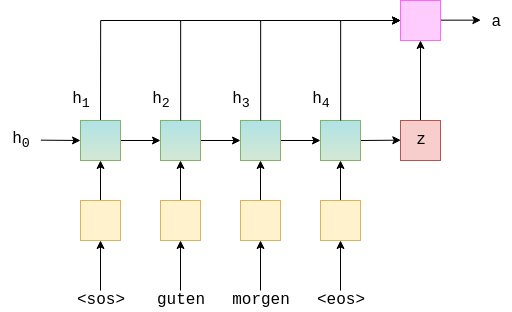
One technical detail here is the use of batch matrix multiplication. Batch matrix multiplication simply treats the first dimension of each vectors as a batch dimension and performs multiplications on the rest of the two dimensions.
\[\text{(batch, k, n)} \times \text{(batch, n, m)} = \text{(batch, k, m)}\]We use batch matrix multiplication in order to calculate the weighted average vector, denoted as $w$ in earlier sections. This entire process can be visualized as follows. $z$ denotes the hidden state of the decoder.
Decoder
This attention network becomes a sub-component of the decoder network, which is shown below.
class Decoder(nn.Module):
    def __init__(
        self,
        vocab_size,
        embed_dim,
        decoder_hidden_size,
        encoder_hidden_size,
        droppout,
    ):
        super(Decoder, self).__init__()
        self.vocab_size = vocab_size
        self.dropout = nn.Dropout(droppout)
        self.embedding = nn.Embedding(vocab_size, embed_dim)
        self.gru = nn.GRU(
            encoder_hidden_size * 2 + embed_dim, decoder_hidden_size
        )
        self.attention = Attention(encoder_hidden_size, decoder_hidden_size)
        self.fc = nn.Linear(
            encoder_hidden_size * 2 + decoder_hidden_size + embed_dim,
            vocab_size
        )

    def forward(self, x, hidden, encoder_outputs):
        x = x.unsqueeze(0)
        # x.shape == (1, batch_size)
        # hidden.shape = (batch_size, decoder_hidden_size)
        embedding = self.dropout(self.embedding(x))
        # embedding.shape == (1, batch_size, embed_dim)
        weighted = self.attention(hidden, encoder_outputs)
        # weighted.shape == (1, batch_size, encoder_hidden_dim * 2)
        weighted_concat = weighted.cat((embedding, weighted), dim=2)
        # weighted_concat.shape == (1, batch_size, encoder_hidden_dim * 2 + embed_dim)
        output, hidden = self.gru(weighted_concat, hidden)
        # output.shape == (1, batch_size, decoder_hidden_size)
        # hidden.shape == (1, batch_size, decoder_hidden_size)
        embedding = embedding.squeeze(0)
        output = output.squeeze(0)
        hidden = hidden.squeeze(0)
        weighted = weighted.squeeze(0)
        # embedding.shape == (batch_size, embed_dim)
        # output.shape == (batch_size, decoder_hidden_size)
        # weighted.shape == (batch_size, encoder_hidden_dim * 2)
        fc_in = torch.cat((output, weighted, embedding), dim=1)
        prediction = self.fc(fc_in)
        # prediction.shape == (batch_size, vocab_size)
        return prediction, hidden
The decoder accepts more components in its forward function. First, it accepts the prediction from the previous decoding time step. This could also be the correct answer labels under a teacher force context. Next, it also accepts the hidden state from the previous decoding time step. Last but not least, it accepts the encoder outputs from all encoding time steps. Note that these encoder outputs are necessary for attention calculation.
In a nutshell, the decoder calculates the weighted average vector using attention, then concatenates this vector with word embeddings. This concatenated vector is then passed to the GRU unit.
We could just use the GRU output for final token predictions, but for extra robustness, we concatenate all vectors that have been produced so far—embedding, attention weighted vector, and the GRU output—all into the final classifier layer. By giving as much information as possible to the classifier, we can minimize the loss of information. These are effectively residual connections.
Seq2Seq
Now, it’s time to put all the pieces together. Below is the final seq2seq model.
class Seq2Seq(nn.Module):
    def __init__(self, encoder, decoder, device):
        super(Seq2Seq, self).__init__()
        self.encoder = encoder
        self.decoder = decoder
        self.device = device

    def forward(self, source, target, teacher_force_ratio=0.5):
        seq_len = target.size(0)
        batch_size = target.size(1)
        outputs = torch.zeros(
            seq_len, batch_size, self.decoder.vocab_size
        ).to(self.device)

        encoder_outputs, hidden = self.encoder(source)
        x = target[0]

        for t in range(seq_len):
            output, hidden = self.decoder(x, hidden, encoder_outputs)
            outputs[t] = output
            teacher_force = random.random() < teacher_force_ratio
            if not teacher_force:
                x = predictions.argmax(1)
            else:
                x = target[t]
        return outputs
If you’ve seen previous seq2seq models we have built in previous posts, you will easily notice that this model is in fact no different from previous models.
Well, this observation is only superficially true. Recall that the main improvement we have implemented in this model is the attention of the attention mechanism, which is currently a sub-component of the decoder. Therefore, this seq2seq model properly uses attention to generate predictions at each decoding time step.
Conclusion
In this post, we explored how attention works, and how one can bake attention into a sequence-to-sequence model. The part that I find most interesting about attention is that it makes so much intuitive sense: when we translate from one language to another, we pay attention to both the overall meaning from the source text as well as the rough one-to-one correspondence between words in source and target languages. Obviously, there are simplifications; most often, humans not only look at individual words or tokens, but also consume phrases or other chunks in the syntax tree. Since this simple seq2seq model has notion of a tree or any hierarchical structure, it can only look at token-to-token correspondence in source and target languages: one time step corresponds to one token. Perhaps in a future post, we will take a look at such more advanced attention mechanisms.
I hope you’ve enjoyed reading this post. Catch you up in the next one!