Recommendation Algorithm with SVD

I’ve been using a music streaming service for the past few weeks, and it’s been a great experience so far. I usually listen to some smoothing new age piano or jazz while I’m working, while I prefer K-pop on my daily commutes and bass-heavy house music during my workouts. Having processed these information through repeated user input on my part, the streaming application now regularly generates playlists each reflective of the three different genres of music that I enjoy most. This got me wondering: what is the underlying algorithm beind content selection and recommendation? How do prominent streaming services such as Netflix and Spotify provide recommendations to their users that seem to reflect their personal preferences and tastes? From a business perspective, these questions carry extreme significance since the accuracy of a recommendation algorithm may directly impact sales revenue.

In this post, we will dive into this question by developing an elementary recommendation engine. The mechanism we will use to achieve this objective is a technique in linear algebra known as singular value decomposition or SVD for short. SVD is an incredibly powerful way of processing data, and also ties in with other important techniques in applied statistics such as principal component analysis, which we might also take a look at in a future post. Enough with the preface, let’s dive right into developing our model.

Singular Value Decomposition

Before we start coding away, let’s first try to understand what singular value decomposition is. In a previous post on Markov chains, we examined the clockwork behind eigendecomposition, a technique used to decompose non-degenerate square matrices. Singular value decomposition is similar to eigendecomposition in that it is a technique that can be used to factor matrices into distinct components. In fact, in deriving the SVD formula, we will later inevitably run into eigenvalues and eigenvectors, which should remind us of eigendecomposition. However, SVD is distinct from eigendecomposition in that it can be used to factor not only square matrices, but any matrices, whether square or rectangular, degenerate or non-singular. This wide applicability is what makes singular decomposition such a useful method of processing matrices.

Now that we have a general idea of what SVD entails, let’s get down into the details.

The SVD Formula

In this section, we take a look at the mathematical clockwork behind the SVD formula. In doing so, we might run into some concepts of linear algebra that requie us to understand some basic the properties of symmetric matrices. The first section is devoted to explaining the formula using these properties; the second section provides explanations and simple proofs for some of the properties that we reference duirng derivation.

Understanding SVD

We might as well start by presenting the formula for singular value decomposition. Given some \(m\)-by-\(n\) matrix \(A\), singular value decomposition can be performed as follows:

\[A = U \Sigma V^{T} \tag{1}\]

There are two important points to be made about formula (1). The first pertains to the dimensions of each factor: \(U \in \mathbb{R}^{m \times m}\), \(\Sigma \in \mathbb{R}^{m \times n}\), \(V \in \mathbb{R}^{n \times n}\). In eigendecomposition, the factors were all square matrices whose dimension was identical to that of the matrix that we sought to decompose. In SVD, however, since the target matrix can be rectangular, the factors are always of the same shape. The second point to note is that \(U\) and \(V\) are orthogonal matrices; \(\Sigma\), a diagonal matrix. This decomposition structure is similar to that of eigendecomposition, and this is no coincidence: in fact, formula (1) can simply be shown by performing an eigendecomposition on \(A^{T}A\) and \(AA^{T}\).

Let’s begin by calculating the first case, \(A^{T}A\), assuming formiula (1). This process looks as follows:

\[A^{T}A = (U \Sigma V^{T})^{T}(U \Sigma V^{T}) = (V \Sigma U^{T})(U \Sigma V^{T}) = V \Sigma^2 V^{T} \tag{2}\]

The last equality stands since the inverse of an orthogonal matrix is equal to its transpose. Substituting \(\Sigma^2\) for \(\Lambda\), equation (2) simplifies to

\[A^{T}A = V \Sigma^2 V^{T} = V \Lambda V^{T} = V \Lambda V^{-1} \tag{3}\]

And we finally have what we have seen with eigendecomposition: a matrix of independent vectors equal to the rank of the original matrix, a diagonal matrix, and an inverse. Indeed, what we have in (3) is an eigendecomposition of the matrix \(A^{T}A\). Intuitively speaking, because matrix \(A\) is not necessarily square, we calculate \(A^{T}A\) to make it square, then perform the familiar eigendecomposition. Note that we have orthogonal eigenvectors in this case because \(A^{T}A\) is a symmetric matrix—more specifically, positive semi-definite. We won’t get into this subtopic too much, but we will explore a very simple proof for this property, so don’t worry. For now, let’s continue with our exploration of the SVD formula by turning our attention from matrix \(V\)—a factor of eigendecomposition on \(A^{T}A\)—to the matrix \(U\).

Much like we understood \(V\) as a factor of eigendecomposition, \(U\) can be seen as a factor of eigendecomposition, this time on the matrix \(AA^T\). Concretly,

\[AA^{T} = (U \Sigma V^{T})(U \Sigma V^{T})^{T} = (U \Sigma V^{T})(V \Sigma U^{T}) = U \Sigma^2 U^T \tag{4}\]

Notice the parallel between (2) and (4). It’s not difficult to see that, by symmetry, \(U\) is also going to be an orthogonal matrix containing the eigenvectors of \(AA^T\). The most important difference between \(U\) and \(V\) concerns dimensionality: while \(U\) is a \(m\)-by-\(m\) matrix, V is an \(n\)-by-\(n\). This disparity originates from the fact that \(A\) itself is a rectangular matrix, meaning that the dimensions of \(AA^{T}\) and \(A^{T}A\) are also different. Another point that requires clarification pertains to \(\Sigma\). Earlier, we made a substitution of \(\Sigma^2\) for \(\Lambda\). This tells us that \(\Sigma\) contains the square roots of the eigenvalues of \(A^{T}A\) and \(AA^T\), which, it is important to note, has identical non-zero eigenvalues. If this point brings confusion, I recommend that you peruse over the next subsection on linear algebra.

Let’s conclude this section with the formula for singular value decomposition:

\[A = U \Sigma V^{T}\]

Hopefully, now it is clear what \(U\), \(\Sigma\), and \(V\) are. Singular value decomposition can intuitively be thought of as a square root version of eigendecomposition, since essentially \(U\) and \(V\) are all derivatives that come from the “square” of a matrix, the two transpose multiples. This intuition also aligns with the fact that \(\Sigma\) is a diagonal matrix containing the square roots of eigenvalues of the transpose products. With these in mind, let’s get ready to build the recommendation model.

Linear Algebra Cheat Sheet

In this optional section, we take a look at two mathematical propositions we referenced while motivating the SVD formula: first, that symmetric matrices have orthogonal eigenvectors; second, that \(A^{T}A\) and \(AA^T\) have identical non-zero eigenvalues. The proof for both of these statements are simple, but feel free to gloss over this section if you just want to see SVD at work instead of the mathematical details behind singular value decomposition.

Eigenvectors of Symmetric Matrices

Let \(A\) be some symmetric matrix, i.e. \(A = A^T\). Also assume that \(A\) has two distinct eigenvectors, \(x\) and \(y\) with corresponding eigenvalues \(\lambda\) and \(\omega\). With this setup, we start from the definition of eigenvectors and eigenvalues:

\[Ax = \lambda x\]

If we apply transpose on both sides,

\[x^{T}A^T = \lambda x^T\]

We can legally multiply both sides by \(y\), which results in the following:

\[x^{T} A^{T}y = \lambda x^{T} y\]

However, since \(A = A^T\),

\[x^{T} Ay = \lambda x^{T} y\]

Furthermore, we can use the fact that the eigenvalue corresponding to \(y\) is \(\omega\). Then,

\[x^{T} Ay = x^{T} \omega y = \omega x^{T}y = \lambda x^{T} y \tag{5}\]

Since \(\lambda \neq \omega\), the only way for (5) to make sense is if \(x^{T}y = 0\)—and this is exactly what we have been trying to show. Since \(x\) and \(y\) are two distinct eigenvectors of the symmetric matrix \(A\), we have successfully shown that any two eigenvectors of \(A\) will be orthogonal, i.e. their dot product is going to be zero.

Eigenvalues of Transpose Products

Let’s start by assuming that \(A^{T}A\) has some non-zero eigenvector \(x\) whose corresponding eigenvalue is \(\lambda\). Then, we have

\[A^{T}Ax = \lambda x\]

If we left multiply both sides by \(A\), we get

\[AA^{T}(Ax) = \lambda (Ax)\]

By the definition of an eigenvector, it is not difficult to see that \(AA^{T}\) has an eigenvector \(Ax\) whose corresponding eigenvalue is \(\lambda\). In short, the reason why SVD works is that the eigenvalue matrix \(\Lambda\) can be obtained either way by performing an eigendecomposition of the matrix \(A^{T}A\) or \(AA^T\).

The Recommendation Algorithm

Now that we have a mathematical understanding of how singular value decomposition, let’s see how we can apply SVD to build a simple recommendation algorithm. This section will continue as follows. First, we examine SVD as a technique of data compression and dimensionality reduction. Next, we generate some toy data of movie reviews and apply SVD to see how we can build a simple function that gives movie recommendations to users given their movie ratings history. Let’s jump right in.

Application of SVD

Why is singular value decomposition so important? Sure, it should now be fairly clear that SVD is a decomposition technique that can be applied to any matrix, whether square or not, which in and of itself makes it a very powerful tool in the statistician’s arsenal. But the true beauty of singular value decomposition comes from the fact that we can perform data compression by extracting meaningful information from the given data. This process is otherwise known as dimensionality reduction, and it is one of the most common applications of singular value decomposition.

Let’s see what this means with an example. Here is \(A\), a target matrix for singuluar value decomposition.

\[A = \begin{pmatrix} 3 & 2 & 2 \\ 2 & 3 & -2 \end{pmatrix}\]

Calculating \(AA^T\), we get

\[AA^T = \begin{pmatrix} 17 & 8 \\ 8 & 17 \end{pmatrix}\]

which is symmetric as we expect. We can calculate the eigenvalues of this matrix by finding the roots of the following characteristic polynomial:

\[det(AA^T - \lambda I) = \lambda^2 - 34\lambda + 225 = (\lambda - 25)(\lambda - 9) = 0\]

Since \(\Sigma\) in SVD is the diagonal matrix that contains the square roots of the eigenvalues of \(AA^T\), we can conclude that

\[\sigma_1 = 5, \sigma_2 = 3\]

where \(\sigma_n\) denotes the value of the \(n\)th diagonal entry in \(\Sigma\). Therefore, given the dimensionality of \(A\), we can conclude that

\[\Sigma = \begin{pmatrix} 5 & 0 & 0 \\ 0 & 3 & 0 \end{pmatrix}\]

Next, we find the eigenvalues of \(AA^T\). This process can be performed by identifying the null space of the matrix \(AA^T - \lambda I\). For instance, given \(\lambda_1 = 25\),

\[AA^T - \lambda_1 I = \begin{pmatrix} -8 & 8 \\ 8 & -8 \end{pmatrix}\]

Given the orientation of this matrix, we see that

\[\begin{pmatrix} \frac{1}{\sqrt 2} \\ \frac{1}{\sqrt 2} \end{pmatrix} \in N(AA^T - \lambda_1 I)\]

By doing the same for \(\lambda_2 = 9\), we can construct the matrix \(U\):

\[U = \begin{pmatrix} \frac{1}{\sqrt 2} & \frac{1}{\sqrt 2} \\ \frac{1}{\sqrt 2} & \frac{-1}{\sqrt 2} \end{pmatrix}\]

Repeating the procedure for \(A^{T}A\) to obtain the factor \(V\), we can complete the singular value decomposition on A:

\[A = \begin{pmatrix} \frac{1}{\sqrt 2} & \frac{1}{\sqrt 2} \\ \frac{1}{\sqrt 2} & \frac{-1}{\sqrt 2} \end{pmatrix} \begin{pmatrix} 5 & 0 & 0 \\ 0 & 3 & 0 \end{pmatrix} \begin{pmatrix} \frac{1}{\sqrt 2} & \frac{1}{\sqrt 2} & 0 \\ \frac{1}{\sqrt 18} & \frac{-1}{\sqrt 18} & \frac{4}{\sqrt 18} \\ \frac{2}{3} & \frac{-2}{3} & \frac{-1}{3} \end{pmatrix}\]

The key to dimensionality reduction is that the first few columns of \(U\), its corresponding eigenvalues in \(\Sigma\), and the corresponding first few rows of \(V^T\) contain the most amount of information on matrix \(A\). As we go down the diagonal entries of \(\Sigma\), we see that the eigenvalues get smaller. The rule of thumb is that the smaller the eigenvalue, the lesser contribution it has on expressing data on \(A\). In other words, we can obtain an approximation of \(A\) by extracting the first few columns and rows of each factor. For example,

\[A \approx \begin{pmatrix} \frac{1}{\sqrt 2} \\ \frac{1}{\sqrt 2} \end{pmatrix} \begin{pmatrix} 5 \end{pmatrix} \begin{pmatrix} \frac{1}{\sqrt 2} & \frac{1}{\sqrt 2} & 0 \end{pmatrix} = \begin{pmatrix} \frac52 & \frac52 & 0 \\ \frac52 & \frac52 & 0 \end{pmatrix}\]

This may seem like a very clumsy way of approximating \(A\). However, this is because the toy matrix we dealt with was a mere two-by-three matrix with only two non-zero entries in the diagonal of \(\Sigma\). Imagine performing the same analysis on a much larger matrix, from which we extract \(r\) number of non-trivial entries of \(\Sigma\). On scale, singular value decomposition becomes more powerful, as it allows large amounts of data to be processed in managable bites.

This is more than enough theory on SVD. Now is finally the time to jump into building our recommendation model with singular value decomposition.

Problem Setup

In this section, we will generate some random data, namely the ratings matrix. The row of the ratings matrix can be interpreted as users; the columns, movies. In other words, \(A_{ij}\) denotes the ratings the \(i\)th user gave for the \(j\)th movie. The example we will use was borrowed from this post by Zacharia Miller.

Let’s quickly build this ratings matrix using numpy and pandas as shown below.

import numpy as np
import pandas as pd

def ratings_matrix(num_users, num_items):
    data = []
    for i in range(num_users):
        user = [np.random.randint(2) for _ in range(num_items)]
        data.append(user)
    mat = pd.DataFrame(data)
    mat.index = ["User " + str(i) for i in range(num_users)]
    mat.columns = ["Movie " + str(i) for i in range(num_items)]
    return mat

Let’s first see what this matrix looks like. We can do this simply by calling the generate_ratings function and saving it to some variable. For notational consistency, let’s name this variable A.

np.random.seed(42)
A = generate_ratings(10, 5)
A

	Movie 0	Movie 1	Movie 2	Movie 3	Movie 4
User 0	0	1	0	0	0
User 1	1	0	0	0	1
User 2	0	0	0	0	1
User 3	0	1	1	1	0
User 4	1	0	1	1	1
User 5	1	1	1	1	1
User 6	0	0	1	1	1
User 7	0	1	0	0	0
User 8	0	0	1	1	1
User 9	1	1	0	1	1

Great! Now we have a matrix of binary numbers, where 1 denotes the fact that the user liked the movie and 0 the fact that they disliked it. We can make some cursory qualitative observations of this toy data. Note, for instance, that users who like Movie 2 also tend to like Movie 3. Also, User 6 and User 8 have identical prefernece for movies—perhaps they both like a particular genre, or tend to like the movie starred by some actor or actress. We would expect singular value decomposition to capture these observations in some way, albeit approximately.

Performing Singular Value Decomposition

Now, let’s actually perform singular value decomposition on the ratings matrix. We could try to do this manually by hand, but let’s utilize the power of modern computing to save ourselves of the time and mental effort involved in calculating the eigenvalues and eigenvectors of a ten-by-ten matrix. Luckily for us, the scipy.linalg module contains some excellent functionality to help us with singular value decomposition. Using this library, singular value decomposition can very simply be achieved with just a few lines of code.

from scipy.linalg import svd

def do_svd(mat, k=0, option=False):
    U, Sigma, VT = svd(mat)
    U = pd.DataFrame(U[:,:k])
    VT = pd.DataFrame(VT[:k,:])
    if option:
        return Sigma
    else:
        return U, VT

The parameters of the do_svd function are mat, the ratings matrix, and k, the number of non-trivial entries of \(\Lambda\) to select for dimensionality reduction, as we have seen earlier. More technically speaking, k corresponds to the number of “concepts” or dimensions that we will extract from the matrix. Let’s see what this means by actually running this function.

U = do_svd(A, 3)[0]
U

	0	1	2
0	-0.070822	-0.457381	-0.098917
1	-0.206427	0.259666	-0.541928
2	-0.125017	0.222040	-0.185270
3	-0.295950	-0.438107	0.440685
4	-0.431556	0.278940	-0.002326
5	-0.502377	-0.178441	-0.101243
6	-0.350146	0.241314	0.354332
7	-0.070822	-0.457381	-0.098917
8	-0.350146	0.241314	0.354332
9	-0.400391	-0.216394	-0.443688

Great! This is what dimensionality reduction means in the loosest sense. Instead of having 5 entries each row, as we had with the original ratings matrix A, we now have 3 entries per row. In other words, the information on users has been compressed into three dimensions. Unlike in A, where each column corresponded to some movie, we don’t really know what the columns of U stand for. It might be some genre, actress, or any hidden patterns in the data set that we are not aware of. Regardless, what’s important here is that we can now understand data more easily in smaller dimensions.

An impotant observation to make is that, as we have noted earlier, User 6 and User 8 have rows that are identical. While this should not be a surprise given that the two users had what seemed to be an identical taste in movies, it is still interesting to see how SVD is able to extract this information and display it onto a new axis.

Next, let’s see what VT looks like.

VT = do_svd(A, 3)[1]
VT.T

	0	1	2
0	-0.354165	0.073549	-0.623270
1	-0.308102	-0.894073	-0.172861
2	-0.443679	0.074189	0.598433
3	-0.535715	-0.036512	0.344539
4	-0.543874	0.434037	-0.323766

Shown above is the transpose of VT, which means that VT.T is just really \({V^T}^T = V\). What’s important here is that the five movies have also been reduced to three dimensions. We don’t really know what the columns of this matrix means; all we know is that it is some distillation and amalgamation of information about the ten users on some unknown axis. At any rate, the previous ten dimensional vectors have now been reduced to three dimensions, which is great news for us—as three dimensional beings, it’s always easier to visualize and deal with three dimensions or less than 10D.

Movie 2 and Movie 3 do not look as similar as they did before on the ratings matrix. However, perhaps this is due to the fact that all entries of this matrix have pretty small values, and it is difficult to see how the difference between Movie 2 and 3 compares to, say, the distance between Movies 1 and 4. Perhaps we should scale this in terms of relative distances or plot it on a three dimensional space, which is exactly what we are going to in a moment.

Before we jump into visualizations, however, let’s deal with the elephant in the room first: is it okay to simply chop off a few dimensions to reduce a high dimensional image to fit into three-dimensional space? To answer this question, let’s check the \(\Sigma\) matrix for this particular instance of singular value decomposition.

do_svd(A, option=True)

array([4.3503838 , 1.95476613, 1.74753126, 0.94245216, 0.55764559])

Note that we already have the first three values of \(\sigma\) in our hands given that k=3 in our instantiation of singular value decomposition. The information we lose pertains to the last two values, given by 0.94245216 and 0.55764559. These values are smaller in order of magnitude compared to, for instance, the largest value of \(\sigma\), which is 4.3503838. This supports the idea that the information we lose amid dimensionality reduction is minimal. Alternatively, we can also see this by taking a look at the full, unreduced version of the matrix \(U\) or \(V\). For example, the code snippet below displays the full version of the factor \(U\).

do_svd(A, 10)[0]

	0	1	2	3	4	5	6	7	8	9
0	-0.070822	-0.457381	-0.098917	0.258014	-0.231719	-4.149231e-01	8.802261e-02	-4.201097e-01	8.802261e-02	-5.399893e-01
1	-0.206427	0.259666	-0.541928	-0.049611	-0.344099	-2.561136e-01	3.357737e-01	-1.030392e-01	3.357737e-01	4.167861e-01
2	-0.125017	0.222040	-0.185270	0.675541	-0.134755	-3.158860e-02	-4.367030e-01	-8.530928e-02	-4.367030e-01	1.911411e-01
3	-0.295950	-0.438107	0.440685	-0.133239	-0.017989	-2.877022e-01	-1.009294e-01	-1.883485e-01	-1.009294e-01	6.079272e-01
4	-0.431556	0.278940	-0.002326	-0.440863	-0.130370	-4.398932e-01	-2.693589e-01	2.957585e-01	-2.693589e-01	-3.138514e-01
5	-0.502377	-0.178441	-0.101243	-0.182849	-0.362089	6.960068e-01	-6.641480e-02	-1.927193e-01	-6.641480e-02	-1.029347e-01
6	-0.350146	0.241314	0.354332	0.284288	0.078975	1.579430e-02	7.183515e-01	4.265464e-02	-2.816485e-01	-9.557056e-02
7	-0.070822	-0.457381	-0.098917	0.258014	-0.231719	6.618514e-03	7.932156e-02	8.011774e-01	7.932156e-02	3.499680e-02
8	-0.350146	0.241314	0.354332	0.284288	0.078975	1.579430e-02	-2.816485e-01	4.265464e-02	7.183515e-01	-9.557056e-02
9	-0.400391	-0.216394	-0.443688	0.029232	0.771458	1.110223e-16	-3.747003e-16	2.775558e-17	-3.747003e-16	-4.440892e-16

It is not difficult to see that the last few columns of \(U\) contain values so small that their contribution to data is going to be minimal at best. This is not the most mathematical way of presenting the concept of data—doing so would require us to take a look at other metrics such as covariance—but this basic analysis will suffice for our purposes for now. The takeaway is that dimensionality reduction is a meaningful way to extract important information from our data.

Now that we have performed SVD on the ratings matrix, let’s move onto the last step: crafting a model for our recommendation algorithm.

The Recommendation Algorithm

My personal pet theory is that using any word in conjunction with “algorithm” makes the concept sound more complex than it actually is. This is exactly what we are doing here, because in reality, our so-called algoithm for movie recommendations is going to be very simple.

The intuition behind the recommendation system is distance calculation. Simply put, if users have similar movie preferences, the points representing the two users will appear to be close when plotted on a graph. Let’s see what this means by plotting U using matplotlib. This can be achieved with the following code.

%matplotlib inline
%config InlineBackend.figure_format = 'retina'
import matplotlib.pyplot as plt
from mpl_toolkits.mplot3d import Axes3D
plt.style.use("seaborn")


def plot_data(mat, data_type, camera=None):
    fig = plt.figure()
    ax = fig.add_subplot(111, projection='3d')
    if camera != None:
        ax.view_init(elev=camera[0], azim=camera[1])
    for index, row in mat.iterrows():
        ax.scatter(row[0], row[1], row[2], alpha=0.8)
        ax.text(row[0], row[1], row[2],'{0} {1}'.format(data_type, index), size=10)
    plt.show()

We can pass U as an argument for the plot_data function to see a three-dimensional plot of users’ movie preferences, as shown below.

plot_data(U, "User")

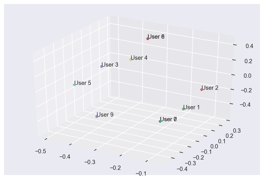
Note that the points corresponding to User 6 and User 8 exactly overlap, which is why the points look darker despite being positioned near the corner of the plot. This is also why we can only count seven points in total despite having plotted eight data points. In short, this visualization shows how we might be able to use distance calculation to give movie recommendations to a new user. Assume, for instance, that we get a new suscriber to our movie application. If we can plot User 10 onto the space above, we will be able to see to whom User 10’s preference is most similar. This comparison is useful since User 10 will most likely like the movie that the other use also rated highly.

We can also create a similar plot for movies instead of users. The plot is shown below:

plot_data(VT.T, "Movie", [-164.5, 51.25])

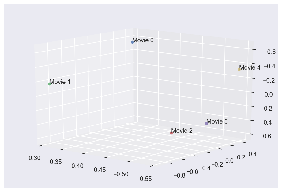
With some alteration of the viewing angle, now we see through visualization that Movies 2 and 3 are close, as we had expected from the original ratings matrix A. This is an interesting result, and it shows just how powerful singular value decomposition is at extracting important patterns from given data sets.

Now that we understand what SVD does for us, it’s time to code our recommender function that uses distance calculation to output movie recommendations. In this post, we will be using the dot product as a means of determining distance, although other metrics such as Euclidean distance would suit our purposes as well. An advantage of using the dot product is that it is computationally less expensive and easy to achieve with code, as shown below.

def recommend(liked_movie, VT, output_num=2):
    global rec
    rec = []
    for item in range(len(VT.columns)):
        if item != liked_movie:
            rec.append([item,np.dot(VT[item],VT[liked_movie])])
    final_rec = [i[0] for i in sorted(rec, key=lambda x: x[1],reverse=True)]
    return final_rec[:output_num]

The recommend function recommends an output_num number of movies given that the user rated liked_movie highly. For example, let’s say some user really liked Movie 2 and is looking for two more movies that are similar to Movie 2. Then, we can simply call the function above by passing in appropriate arguments as follows.

recommend(2, VT)

[3, 4]

This function tells us that our movie application should recommend to our user Movies 3 and 4, in that order. This result is not surprising given the fact that we have already observed the closeness between Movies 2 and 3—if a user likes Movie 2, we should definitely recommend Movie 3 to them. Our algorithm also tells us that the distance between Movie 2 and 4 is also pretty close, although not as close as the distance between Movies 2 and 3.

What is happening behind the scene here? Our function simply calculates the distance between the vector representation of each movies as a dot product. If we were to print the local variable rec array defined within the recommend function, for instance, we would see the following result.

rec

[[0, -0.21039350295933443],
 [1, -0.033077064237217],
 [3, 0.4411602025458312],
 [4, 0.07975391765448048]]

This tells us how close Movies 0, 1, 3, and 4 are with Movie 2. The larger the dot product, the closer the movie; hence, the more compelling that recommendation. The recommend function then sorts the rec array and outputs the first output_num movies as a recommendation. Of course, we could think of an alternate implementation of this algorithm that makes use of the U matrix instead of VT, but that would be a slightly different recommendation system that uses past user’s movie ratings as information to predict whether or not the particular individual would like a given movie. As we can see, SVD can be used in countless ways in the domain of recommendation algorithms, which goes to show how powerful it is as a tool for data analysis.

Conclusion

In today’s post, we dealt primarily with singular value decomposition and its application in the context of recommendation systems. Although the system we built in this post is extremely simple, especially in comparison to the complex models that companies use in real-life situations, nonetheless our exploration of SVD is valuable in that we started from the bare basics to build our own model. What is even more fascinating is that many recommendation systems involve singular value decomposition in one way or another, meaning that our exploration is not detached from the context of reality. Hopefully this post has given you some intuition behind how recommendation systems work and what math is involved in those algorithms.

On a tangential note, recently, I have begun to realize that linear algebra as a university subject is very different from linear algebra as a field of applied math. Although I found interest in linear algebra last year when I took the course as a first-year, studying math on my own has endowed me with a more holistic understanding of how the concepts and formulas we learned in linear algebra class can be used in real-life contexts. While I am no expert in pedagogy or teaching methodology, this makes me believe that perhaps linear algebra could be taught better if students were exposed to applications with appropriate data to toy around with. Just a passing thought.

Anyhow, that’s enough blogging for today. Catch you up in the next one.