Markov Chain and Chutes and Ladders
In a previous post, we briefly explored the notion of Markov chains and their application to Google’s PageRank algorithm. Today, we will attempt to understand the Markov process from a more mathematical standpoint by meshing it together the concept of eigenvectors. This post was inspired and in part adapted from this source.
Revisiting Eigenvectors
In linear algebra, an eigenvector of a linear transformation is roughly defined as follows:
a nonzero vector that is mapped by a given linear transformation onto a vector that is the scalar multiple of itself
This definition, while seemingly abstract and cryptic, distills down into a simple equation when written in matrix form:
\[Ax = \lambda x\]Here, \(A\) denotes the matrix representing a linear transformation; \(x\), the eignevector; \(\lambda\), the scalar value that is multiplied onto the eigenvector. Simply put, an eigenvector \(x\) of a linear transformation is one that is—allow me to use this term in the loosest sense to encompass positive, negative, and even imaginary scalar values—“stretched” by some factor \(\lambda\) when the transformation is applied, i.e. multiplied by the matrix \(A\) which maps the given linear transformation.
The easiest example I like to employ to demonstrate this concept is the identity matrix \(I\). For the purpose of demonstration, let \(a\) be an arbritrary vector \((x, y, z)^{T}\) and \(I\) the three-by-three identity matrix. Multiplying \(a\) by \(I\) produces the following result:
\[Ia = \begin{pmatrix} 1 & 0 & 0 \\ 0 & 1 & 0 \\ 0 & 0 & 1 \end{pmatrix} \begin{pmatrix} x \\ y \\ z \end{pmatrix} = \begin{pmatrix} x \\ y \\ z \end{pmatrix}\]The result is unsurprising, but it reveals an interesting way of understanding \(I\): identity matrices are a special case of diagonalizable matrices whose eigenvalues are 1. Because the multiplying any arbitrary vector by the identity matrix returns the vector itself, all vectors in the dimensional space can be considered an eigenvector to the matrix \(I\), with \(\lambda\) = 1.
A formal way to calculate eigenvectors and eigenvalues can be derived from the equation above.
\[Ax = \lambda x\] \[Ax - \lambda x = 0\] \[(A - \lambda I)x = 0\]Since \(x\) is assumed as a nonzero vector, we can deduce that the matrix \((A - \lambda I)\) is a singular matrix with a nontrivial null space. In fact, the vectors in this null space are precisely the eigenvectors that we are looking for. Here, it is useful to recall that the a way to determine the singularity of a matrix is by calculating its determinant. Using these set of observations, we can modify the equation above to the following form:
\[det(A - \lambda I) = 0\]By calculating the determinant of \((A - \lambda I)\), we can derive the characteristic polynomial, from which we can obtain the set of eigenvectors for \(A\) representing some linear transformation \(T\).
Constructing the Stochastic Matrix
Now that we have reviewed some underlying concepts, perhaps it is time to apply our knowledge to a concrete example. Before we move on, I recommend that you check out this post I have written on the Markov process, just so that you are comfortable with the material to be presented in this section.
In this post, we turn our attention to the game of Chutes and Ladders, which is an example of a Markov process which demonstrates the property of “memorylessness.” This simply means that the progress of the game depends only on the players’ current positions, not where they were or how they got there. A player might have ended up where they are by taking a ladder or by performing a series of regular dice rolls. In the end, however, all that matters is that the players eventually hit the hundredth cell.
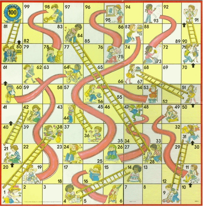
To perform a Markov chain analysis on the Chutes and Ladders game, it is first necessary to convert the information presented on the board as a stochastic matrix. How would we go about this process? Let’s assume that we start the game at the \(0\)th cell by rolling a dice. There are six possible events, each with probability of \(1/6\). More specifically, we can end up at the index numbers 38, 2, 3, 14, 5, or 6. In other words, at position 0,
\[P(X = x \vert C = 0) = \begin{cases} \ \frac 16 & \{x \vert x \in 38, 2, 3, 14, 5, 6\} \\[2ex] \ 0 & \{x \vert x \notin 38, 2, 3, 14, 5, 6\} \end{cases}\]where \(C\) and \(X\) denote the current and next position of the player on the game board, respectively. We can make the same deductions for other cases where \(C = 1 \ldots 100\). We are thus able to construct a 101-by-101 matrix representing the transition probabilities of our Chutes and Ladders system, where each column represents the system at a different state, i.e. the \(j\)th entry of the \(i\)th column vector represents the probabilities of moving from cell \(i\) to cell \(j\). To make this more concrete, let’s consider a program that constructs the stochastic matrix T_1, without regards to the chutes and ladders for now.
import numpy as np
import matplotlib.pyplot as plt

def stochastic_mat(dim=101):
"""Returns a 2D numpy stochastic matrix."""

    # Initialize ndarray of zeros
    T_1 = np.zeros((dim, dim))

    # Assign probability to appropriate entries
    for i in range(101):
        if i < 95:
            T_1[i + 1:i + 1 + roll, i] = 1. / roll
        elif i != 100:
            T_1[i + 1:100, i] = 1. / roll
            T_1[100, i] = 1 - (1. / roll) * (99 - i)
        else:
            T_1[i, i] = 1.

    return T_1
The indexing is key here: for each column, \([i + 1, i + 7)\)th rows were assigned the probability of \(1/6\). Let’s say that a player is in the \(i\)th cell. Assuming no chutes or ladders, a single roll of a dice will place him at one of the cells from \((i + 1)\) to \((i + 6)\); hence the indexing as presented above. However, this algorithm has to be modified for i bigger or equal to 95. For example if i == 97, there are only three probabilities: \(P(X = 98)\), \(P(X = 99)\), and \(P(X = 100)\), each of values \(1/6\), \(1/6\), and \(2/3\) respectively. The else statements are additional corrective mechanisms to account for this irregularity. So now we’re done with the stochastic matrix!
… or not quite.
Things get a bit more complicated once we throw the chutes and ladders into the mix. To achieve this, we first build a dictionary containing information on the jump from one cell to another. In this dictionary, the keys correspond to the original position; the values, the index of the cell after the jump, either through a chute or a ladder.
chutes_ladders = {
1: 38, 4: 14, 9: 31, 16: 6, 21: 42,
28: 84, 36: 44, 47: 26, 49: 11, 51: 67,
56: 53, 62: 19, 64: 60, 71: 91, 80: 100,
87: 24, 93: 73, 95: 75, 98: 78
}
For example, 1: 38 represents the first ladder on the game board, which moves the player from the first cell to the thirty eighth cell.
To integrate this new piece of information into our code, we need to build a permutation matrix that essentially “shuffles up” the entries of the stochastic matrix T_1 in such a way that the probabilities can be assigned to the appropriate entries. For example, T_1 does not reflect the fact that getting a 1 on a roll of the dice will move the player up to the thirty eighth cell; it supposes that the player would stay on the first cell. The new permutation matrix T_2 would adjust for this error by reordering T_1. For an informative read on the mechanics of permutation, refer to this explanation from Wolfram Alpha.
# Initialize ndarray of zeros
T_2 = np.zeros((dim, dim))

# ndarray of 101 elements
# If i in chutes_ladders, replace i with corresponding value
index_lst = [chutes_ladders.get(j, j) for j in range(101)]

# Permutation matrix
T_2[index_lst, range(101)] = 1
Let’s perform a quick sanity check to verify that T_2 contains the right information on the first ladder, namely the entry 1: 38 in the chutes_ladders dictionary.
>>> print(T_2[:, 1])
>>> [0. 0. 0. 0. 0. 0. 0. 0. 0. 0. 0. 0. 0. 0. 0. 0. 0. 0. 0. 0. 0. 0. 0. 0.
 0. 0. 0. 0. 0. 0. 0. 0. 0. 0. 0. 0. 0. 0. 1. 0. 0. 0. 0. 0. 0. 0. 0. 0.
 0. 0. 0. 0. 0. 0. 0. 0. 0. 0. 0. 0. 0. 0. 0. 0. 0. 0. 0. 0. 0. 0. 0. 0.
 0. 0. 0. 0. 0. 0. 0. 0. 0. 0. 0. 0. 0. 0. 0. 0. 0. 0. 0. 0. 0. 0. 0. 0.
 0. 0. 0. 0. 0.]
Notice the \(1\) in the \(38\)th entry hidden among a haystack of 100 \(0\)s! This result tells us that T_2 is indeed a permutation matrix whose multiplication with T_1 will produce the final stochastic vector that correctly enumerates the probabilities encoded into the Chutes and Ladders game board. Here is our final product:
import numpy as np
import matplotlib.pyplot as plt

def stochastic_mat(dim=101):

    chutes_ladders = {
    1: 38, 4: 14, 9: 31, 16: 6, 21: 42,
    28: 84, 36: 44, 47: 26, 49: 11, 51: 67,
    56: 53, 62: 19, 64: 60, 71: 91, 80: 100,
    87: 24, 93: 73, 95: 75, 98: 78
    }

    T_1 = np.zeros((dim, dim))
    T_2 = np.zeros((dim, dim))

    for i in range(101):
        if i < 95:
            T_1[i + 1:i + 1 + roll, i] = 1. / roll
        elif i != 100:
            T_1[i + 1:100, i] = 1. / roll
            T_1[100, i] = 1 - (1. / roll) * (99 - i)
        else:
            T_1[i, i] = 1.

    index_lst = [chutes_ladders.get(j, j) for j in range(101)]

    T_2[index_lst, range(101)] = 1

    T = T_2 @ T_1

    return T
We can visualize the stochastic matrix \(T\) using the matplotlib package.
T = stochastic_mat()
plt.matshow(T)
plt.show()
This produces a visualization of our stochastic matrix.
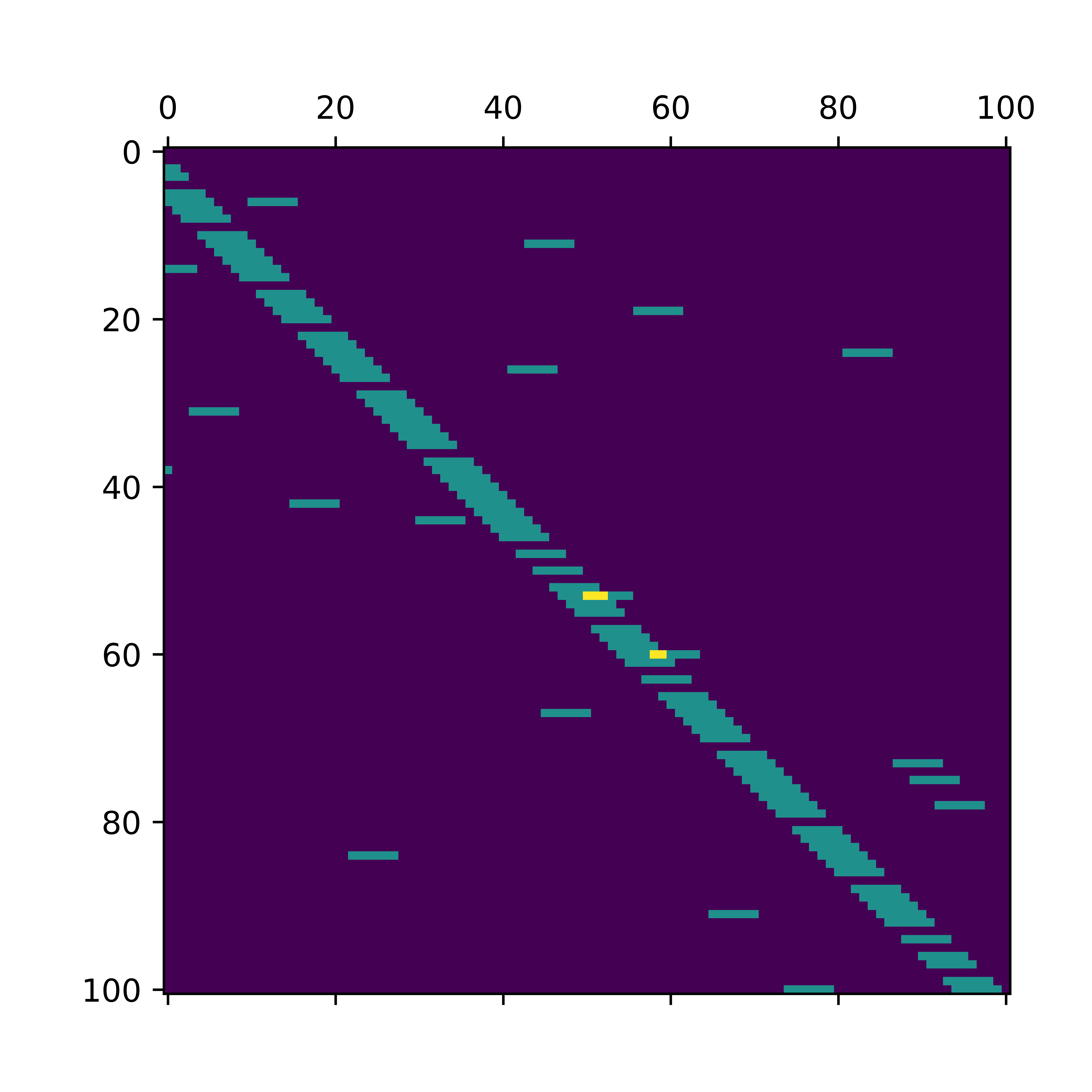
So there is our stochastic matrix!
Stationary Distribution
Now that we have a concrete matrix to work with, let’s start by identifying its eigenvectors. This step is key to understanding Markov processes since the eigenvector of the stochastic matrix whose eigenvalue is 1 is the stationary distribution vector, which describes the Markov chain in a state of equilibrium. For an intuitive explanation of this concept, refer to this previous post.
Let’s begin by using the numpy package to identify the eigenvalues and eigenvectors of the stochastic matrix.
e_val, e_vec = np.linalg.eig(T)
print(e_val[:, 10])
This code block produces the following output:
[1.        +0.j         0.        +0.j         0.95713536+0.j
 0.39456672+0.65308575j 0.39456672-0.65308575j 0.7271442 +0.j
 0.5934359 +0.32633782j 0.5934359 -0.32633782j 0.24218551+0.59481026j
 0.24218551-0.59481026j]
The first entry of this array, which is the value 1. + 0.j, deserves our attention, as it is the eigenvalue which corresponds to the stationary distribution eigenvector. Since the index of this value is 0, we can identify its eigenvector as follows:
>>> e_vec[:, 0]
>>> [0.+0.j 0.+0.j 0.+0.j 0.+0.j 0.+0.j 0.+0.j 0.+0.j 0.+0.j 0.+0.j 0.+0.j
 0.+0.j 0.+0.j 0.+0.j 0.+0.j 0.+0.j 0.+0.j 0.+0.j 0.+0.j 0.+0.j 0.+0.j
 0.+0.j 0.+0.j 0.+0.j 0.+0.j 0.+0.j 0.+0.j 0.+0.j 0.+0.j 0.+0.j 0.+0.j
 0.+0.j 0.+0.j 0.+0.j 0.+0.j 0.+0.j 0.+0.j 0.+0.j 0.+0.j 0.+0.j 0.+0.j
 0.+0.j 0.+0.j 0.+0.j 0.+0.j 0.+0.j 0.+0.j 0.+0.j 0.+0.j 0.+0.j 0.+0.j
 0.+0.j 0.+0.j 0.+0.j 0.+0.j 0.+0.j 0.+0.j 0.+0.j 0.+0.j 0.+0.j 0.+0.j
 0.+0.j 0.+0.j 0.+0.j 0.+0.j 0.+0.j 0.+0.j 0.+0.j 0.+0.j 0.+0.j 0.+0.j
 0.+0.j 0.+0.j 0.+0.j 0.+0.j 0.+0.j 0.+0.j 0.+0.j 0.+0.j 0.+0.j 0.+0.j
 0.+0.j 0.+0.j 0.+0.j 0.+0.j 0.+0.j 0.+0.j 0.+0.j 0.+0.j 0.+0.j 0.+0.j
 0.+0.j 0.+0.j 0.+0.j 0.+0.j 0.+0.j 0.+0.j 0.+0.j 0.+0.j 0.+0.j 0.+0.j
 1.+0.j]
Notice that this eigenvector is a representation of a situation in which the player is in the \(100\)th cell of the game board! In other words, it is telling us that once the user reaches the \(100\)th cell, they will stay on that cell even after more dice rolls—hence the stationary distribution. On one hand, this information is impractical given that a player who reaches the end goal will not continue the game to go beyond the \(100\)th cell. On the other hand, it is interesting to see that the eigenvector reveals information about the structure of the Markov chain in this example.
Markov chains like these are referred to as absorbing Markov chains because the stationary equilibrium always involves a non-escapable state that “absorbs” all other states. One might visualize this system as having a loop on a network graph, where it is impossible to move onto a different state because of the circular nature of the edge on the node of the absorbing state.
A Note on Eigendecomposition
At this point, let’s remind ourselves of the end goal. Since we have successfully built a stochastic matrix, all we have to do is to set some initial starting vector \(x_0\) and perform iterative matrix calculations. In recursive form, this statement can be expressed as follows:
\[x_{n+1} = Tx_n = T^{n+1}x_0\]The math-inclined thinkers in this room might consider the possibility of conducting an eigendecomposition on the stochastic matrix to simply the calculation of matrix powers. There is merit to considering this proposition, although later on we will see that this approach is inapplicable to the current case.
Eigendecomposition refers to a specific method of factorizing a matrix in terms of its eigenvalues and eigenvectors. Let’s begin the derivation: let \(A\) be the matrix of interest, \(S\) a matrix whose columns are eigenvectors of \(A\), and \(\Lambda\), a matrix whose diagonal entries are the corresponding eigenvalues of \(S\).
Let’s consider the result of multiplying \(A\) and \(S\). If we view multiplication as a repetition of matrix-times-vector operations, we yield the following result.
\[AS = A \cdot \begin{pmatrix} \vert & \vert & & \vert \\ s_1 & s_2 & \ldots & s_n \\ \vert & \vert & & \vert \end{pmatrix} = \begin{pmatrix} \vert & \vert & & \vert \\ As_1 & As_2 & \ldots & As_n \\ \vert & \vert & & \vert \end{pmatrix}\]But recall that \(s\) are eigenvectors of \(A\), which necessarily implies that
\[As_n = \lambda s_n\]Therefore, the result of \(AS\) can be rearranged and unpacked in terms of \(\Lambda\):
\(\begin{pmatrix} \vert & \vert & & \vert \\ As_1 & As_2 & \ldots & As_n \\ \vert & \vert & & \vert \end{pmatrix} = \begin{pmatrix} \vert & \vert & & \vert \\ \lambda_1 s_1 & \lambda_2 s_2 & \ldots & \lambda_n s_n \\ \vert & \vert & & \vert \end{pmatrix}\) \(= \begin{pmatrix} \vert & \vert & & \vert \\ s_1 & s_2 & \ldots & s_n \\ \vert & \vert & & \vert \end{pmatrix} \begin{pmatrix} \lambda_1 & \dots & 0 \\ \vdots & \ddots & \vdots \\ 0 & \dots & \lambda_n \end{pmatrix} = S \Lambda\)
In short,
\[AS = S \Lambda\] \[ASS^{-1} = A = S \Lambda S^{-1}\]Therefore, we have \(A = S \Lambda S^{-1}\), which is the formula for eigendecomposition of a matrix.
One of the beauties of eigendecomposition is that it allows us to compute matrix powers very easily. Concretely,
\[A^n = {(S \Lambda S^{-1})}^n = (S \Lambda S^{-1}) \cdot (S \Lambda S^{-1}) \dots (S \Lambda S^{-1}) = S \Lambda^n S^{-1}\]Because \(S\) and \(S^{-1}\) nicely cross out, all we have to compute boils down to \(\Lambda^n\)! This is certainly good news for us, since our end goal is to compute powers of the stochastic matrix to simulate the Markov chain. However, an important assumption behind eigendecomposition is that it can only be performed on nonsingular matrices. Although we won’t go into the formal proofs here, having a full span of independent eigenvectors implies full rank, which is why we must check if the stochastic matrix is singular before jumping into eigendecomposition.
>>> print(np.linalg.matrix_rank(T))
>>> 81
Unfortunately, the stochastic matrix is singular because \(81 < 101\), the number of columns or rows. This implies that our matrix is degenerate, and that the best alternative to eigendecomposition is the singular value decomposition. But for the sake of simplicity, let’s resort to the brute force calculation method instead and jump straight into some statistical analysis.
Simulating Chutes and Ladders
We first write a simple function that simulates the Chutes and Ladders game given a starting position vector v_0. Because a game starts at the \(0\)th cell by default, the function includes a default argument on v_0 as shown below:
def game_simulate(n, T=stochastic_mat(), v_0=[1, *np.zeros(100)]):
'''Returns probability vector'''
    return np.linalg.matrix_power(T, n) @ v_0
Calling this function will give us \(T^nx_0\), which is a 101-by-1 vector whose ith entry represents the probability of the player being on the \(i\)th cell after a single turn. Now, we can plot the probability distribution of the random variable \(N\), which represents the number of turns necessary for a player to end the game. This analysis can be performed by looking at the values of game_simulate(n)[-1] since the last entry of this vector encodes the probability of the player being at the \(100\)th cell, i.e. successfully completing the game after n rounds.
percent_dist = [game_simulate(n)[-1] * 100 for n in range(300)]

plt.plot(np.arange(300), percent_dist)
plt.grid(True)
plt.title('Cumulative Game Completion Rate')
plt.xlabel('Number of Turns')
plt.ylabel('% of Games Completed')
plt.show()
This block produces the following figure:
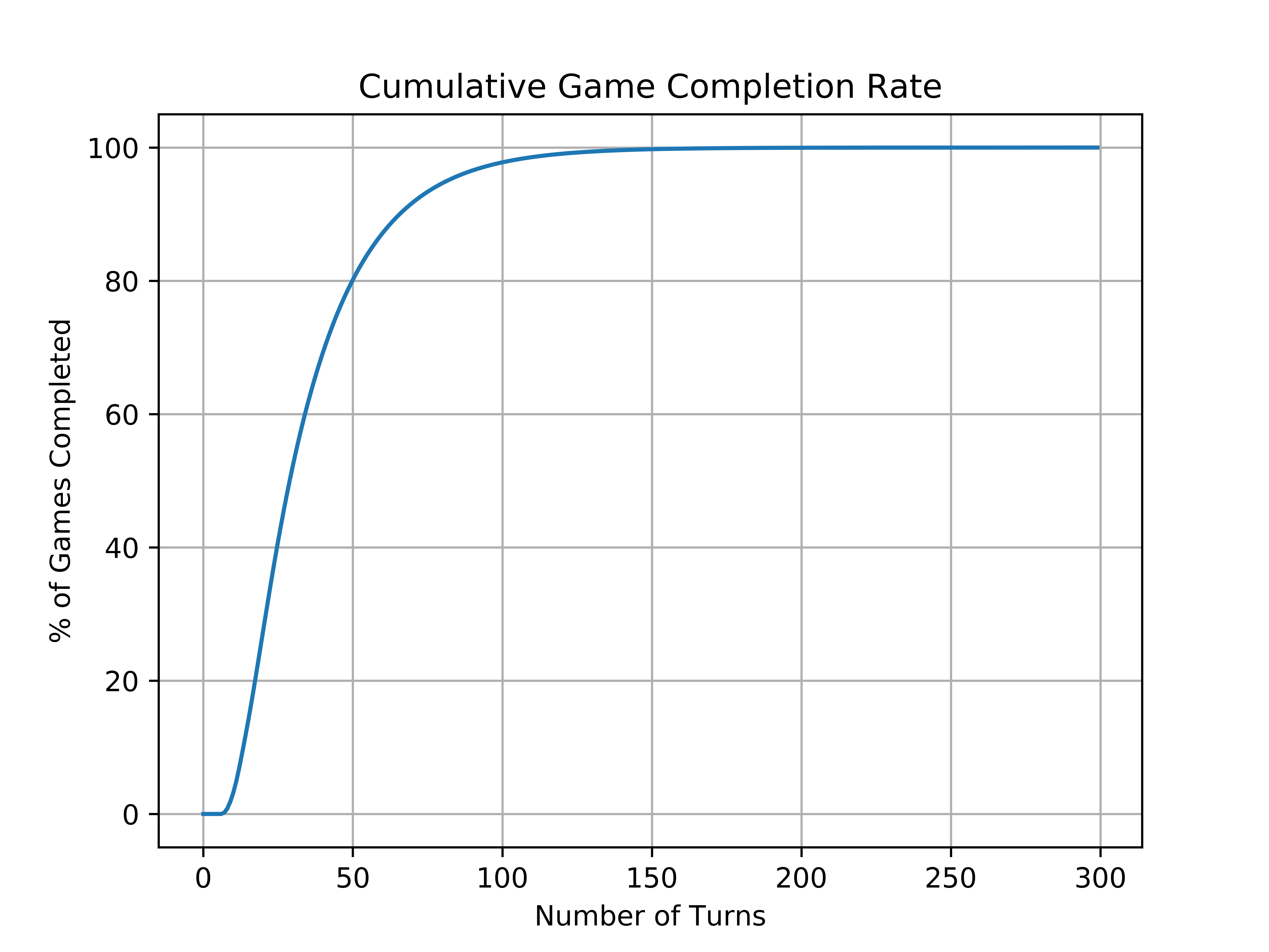
I doubt that anyone would play Chutes and Ladders for this long, but after about 150 rolls of the dice, we can expect with a fair amount of certainty that the game will come to an end.
The graph above presents information on cumulative fractions, but we can also look at the graph for marginal probabilities by examining its derivative:
prob_dist = [game_simulate(n)[-1] for n in range(200)]

plt.plot(np.diff(prob_dist))
plt.grid(True)
plt.title('Marginal Game Completion Rate')
plt.xlabel('Number of Turns')
plt.ylabel('Fraction of Games Completed')
plt.show()
And the result:
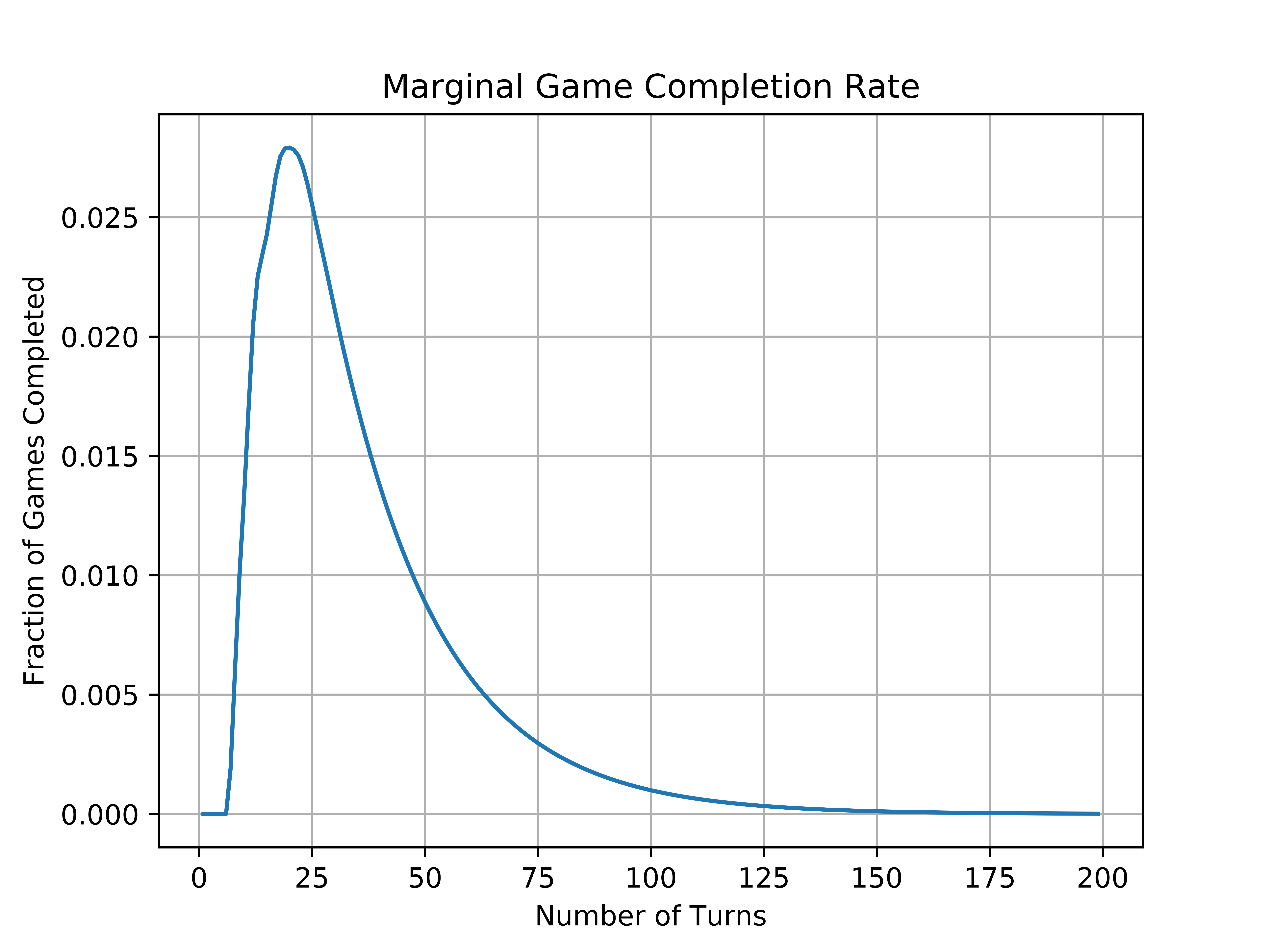
From the looks of it, the maximum of the graph seems to exist somewhere around \(n = 20\). To be exact, \((x_{max}, y_{max}) = (19, 0.027917820873612303)\).
>>> print(np.argmax(np.diff(prob_dist)))
>>> 19
>>> print(np.diff(prob_dist)[19])
>>> 0.027917820873612303
This result tells us that we will finish the game in 19 rolls of the dice more often than any other number of turns.
Typical Game Length
We can also use this information to calculate the expected value of the game length. Recall that
\[E(X) = \sum x_i \cdot P(X = x_i)\]Or if the probability density function is continuous,
\[E(X) = \int x_i \cdot P(X = x_i)\]In this case, we have a discrete random variable, so we adopt the first formula for our analysis. The formula can be achieved in Python as follows:
turns = np.arange(1, len(prob_dist))
exp_val = np.dot(turns, np.diff(prob_dist))
>>> print(exp_val)
>>> 35.77043547952134
This result tells us that the typical length of a Chutes and Ladders game is approximately 36 turns. But an issue with using expected value as a metric of analysis is that long games with infinitesimal probabilities are weighted equally to short games of substantial probability of occurrence. This mistreatment can be corrected for by other ways of understanding the distribution, such as median:
>>> print(prob_dist.index(min(prob_dist, key=lambda x:abs(x-0.5))))
>>> 29
This function tries to find the point in the cumulative distribution where the value is closest to \(0.5\), i.e. the median of the distribution. The result tells us that about fifty percent of the games end after 29 turns. Notice that this number is smaller than \(E(X)\) because it discredits more of the long games with small probabilities.
Conclusion
The Markov chain represents an in interesting way to analyze systems that are memoryless, such as the one in today’s post, the Chutes and Ladders game. Although it is a simple game, it is fascinating to see just how much information and data can be derived from a simple image of the game board. In a future post, we present another way to approach similar systems, known as Monte Carlo simulations. But that’s for another time. Peace!