Linear Regression, in Two Ways

If there is one thing I recall most succinctly from my high school chemistry class, it is how to use Excel to draw basic plots. In the eyes of a naive freshman, visualizations seemed to add an air of professionalism. So I would always include a graph of some sort in my lab report, even when I knew they were superfluous. The final icing on the cake? A fancy regression with some r-squared.

In today’s post, I want to revisit what used to be my favorite tinkering toy in Excel: regression. More specifically, we’ll take a look at linear regression, which deals with straight lines and planes instead of curved surfaces. Although it sounds simple, the linear regression model is still widely used because it not only provides a clearer picture of obtained data, but can also be used to make predictions based on previous observations. Linear regression is also incredibly simple to implement using existing libraries in programming languages such as Python, as we will later see in today’s post. That was a long prologue—–let’s jump right in.

Back to Linear Algebra

In this section, we will attempt to frame regression in linear algebra terms and use basic matrix operations to derive an equation for the line of best fit.

Problem Setup

In this section, we will use linear algebra to understand regression. An important theme in linear algebra is orthogonality. How do we determine if two vectors—or more generally, two subspaces—are orthogonal to each other? How do we make two non-orthogonal vectors orthogonal? (Hence Gram-Schmidt.) In our case, we love orthogonality because they are key to deriving the equation for the line of best fit through projection. To see what this means, let’s quickly assume a toy example to work with: assume we have three points, \((1, 1), (2, 2)\) and \((3, 2)\), as shown below.

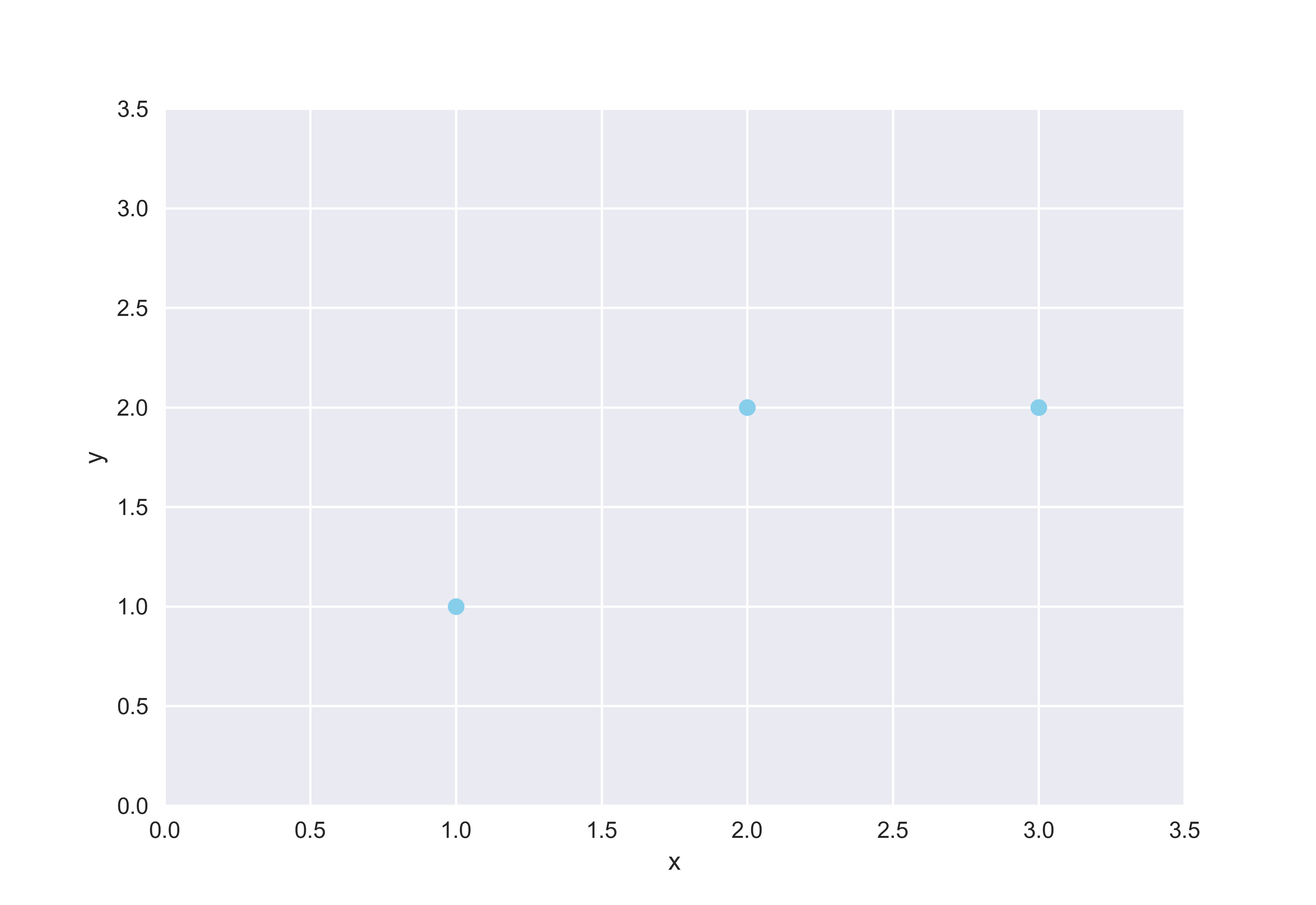
As we can see, the three points do not form a single line. Therefore, it’s time for some regression. Let’s assume that this line is defined by \(y = ax + b\). The system of equations which we will attempt to solve looks as follows:

\[\begin{cases} a + b = 1 \\ 2a + b = 2 \\ 3a + b = 2 \end{cases}\]

Or if you prefer the vector-matrix representation as I do,

\[\underbrace{\begin{pmatrix} 1 & 1 \\ 2 & 1 \\ 3 & 1 \end{pmatrix}}_{A} \underbrace{\begin{pmatrix} x \\ 1 \end{pmatrix}}_{x} = \underbrace{\begin{pmatrix} 1 \\ 2 \\ 2 \end{pmatrix}}_{y}\]

This system, remind ourselves, does not have a solution because we have geometrically observed that no straight line can pass through all three points. What we can do, however, is find a projection of the vector \(y\) onto matrix \(A\) so that we can identify a solution that is closest to \(y\), which we shall denote as \(\hat{y}\). As you can see, this is where all the linear algebra kicks in.

Deriving the Projection Formula

Let’s start by thinking about \(\hat{y}\), the projection of \(y\) onto \(A\). After some thinking, we can convince ourselves that \(\hat{y}\) is the component of \(y\) that lives within the column space of \(A\), and that \(y - \hat{y}\) is the error component of \(y\) that lives outside the column space of \(A\). From this, it follows that \(y - \hat{y}\) is orthogonal to \(C(A)\), since any non-orthogonal component would have been factored into \(\hat{y}\). Concretely,

\[A^{T}(y - \hat{y}) = 0\]

since the transpose is an alternate representation of the dot product. We can further specify this equation by using the fact that \(\hat{y}\) can be expressed as a linear combination of the columns of \(A\). In other words,

\[A^{T}(y - A\hat{x}) = 0 \tag{1}\]

where \(\hat{x}\) is the solution to the system of equations represented by \(Ax = \hat{y}\). Let’s further unpackage (1) using matrix multiplication.

\[A^{T}y - A^{T}A\hat{x} = 0\]

Therefore,

\[A^{T}y = A^{T}A\hat{x}\]

We finally have a formula for \(\hat{x}\):

\[\hat{x} = (A^{T}A)^{-1}A^{T}y \tag{2}\]

Let’s remind ourselves of what \(\hat{x}\) is and where we were trying to get at with projection in the context of regression. We started off by plotting three data points, which we observed did not form a straight line. Therefore, we set out to identify the line of best fit by expressing the system of equations in matrix form, \(Ax = y\), where \(x = (a, b)^{T}\). But because this system does not have a solution, we ended up modifying the problem to \(Ax = \hat{y}\), since this is as close as we can get to solving an otherwise unsolvable system. So that’s where we are with equation (2): a formula for \(\hat{x}\), which contains the parameters that define our line of best fit. Linear regression is now complete. It’s time to put our equation to the test by applying it to our toy data set.

Testing the Formula

Let’s apply (2) in the context of our toy example with three data points to perform a quick sanity check. Calculating the inverse of \(A_{T}A\) is going to be a slight challenge, but this process is going to be a simple plug-and-play for the most part. First, let’s remind ourselves of what \(A\) and \(y\) are:

\[A = \begin{pmatrix} 1 & 1 \\ 2 & 1 \\ 3 & 1 \end{pmatrix}, y = \begin{pmatrix} 1 \\ 2 \\ 2 \end{pmatrix}\]

Let’s begin our calculation:

\[A^{T}A = \begin{pmatrix} 1 & 2 & 3 \\ 1 & 1 & 1 \end{pmatrix} \begin{pmatrix} 1 & 1 \\ 2 & 1 \\ 3 & 1 \end{pmatrix} = \begin{pmatrix} 14 & 6 \\ 6 & 3 \end{pmatrix}\]

Calculating the inverse,

\[(A^{T}A)^{-1} = \begin{pmatrix} \frac12 & -1 \\ -1 & \frac{7}{3} \end{pmatrix}\]

Now, we can put this all together.

\[(A^{T}A)^{-1}A^{T}y = \begin{pmatrix} \frac12 & -1 \\ -1 & \frac73 \end{pmatrix} \begin{pmatrix} 1 & 2 & 3 \\ 1 & 1 & 1 \end{pmatrix} \begin{pmatrix} 1 \\ 2 \\ 2 \end{pmatrix} \\ = \begin{pmatrix} \frac12 & -1 \\ -1 & \frac73 \end{pmatrix} \begin{pmatrix} 11 \\ 5 \end{pmatrix} = \begin{pmatrix} \frac12 \\ \frac23 \end{pmatrix}\]

The final result tells us that the line of best fit, given our data, is

\[y = \frac12 x + \frac23\]

Let’s plot this line alongside our toy data to see how the equation fits into the picture.

import matplotlib.pyplot as plt
import numpy as np
plt.style.use("seaborn")

data = [(1, 1), (2, 2), (3, 2)]
x, y = zip(*data)
plt.scatter(x, y, color="skyblue")
plt.plot(np.linspace(0, 5, 50), 0.5*np.linspace(0, 5, 50) + 2/3, color="skyblue")
plt.xlabel("x"); plt.ylabel("y")
plt.xlim(0, 3.5); plt.ylim(0, 3.5)
plt.show()

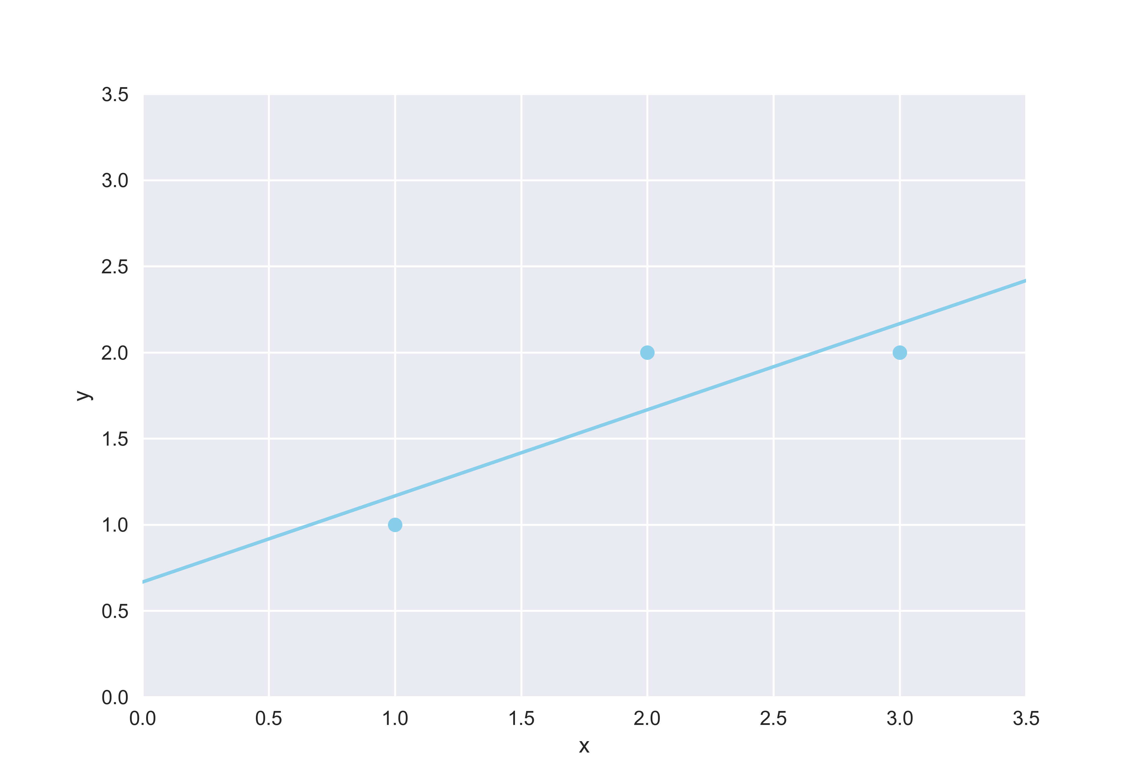
It’s not difficult to see that linear regression was performed pretty well as expected. However, ascertaining the accuracy of a mathematical model with just a quick glance of an eye should be avoided. This point then begs the question: how can we be sure that our calculated line is indeed the best line that minimizes error? To that question, matrix calculus holds the key.

Matrix Calculus

We all remember calculus from school. We’re not going to talk much about calculus in this post, but it is definitely worth mentioning that one of the main applications of calculus lies in optimization: how can we minimize or maximize some function, optionally with some constraint? This particular instance of application is particularly pertinent and important in our case, because, if we think about it, the linear regression problem can also be solved with calculus. The intuition behind this approach is simple: if we can derive a formula that expresses the error between actual values of \(y\) and those predicted by regression, denoted as \(\hat{y}\) above, we can use calculus to derive that expression and ultimately locate the global minimum. And that’s exactly what we’re going to do.

But before we jump into it, let’s briefly go over some basics of matrix calculus, which is the variant of calculus we will be using throughout.

The Gradient

Much like we can derive a function by a variable, say \(x\) or \(y\), loosely speaking, we can derive a function by a matrix. More strictly speaking, this so-called derivative of a matrix is more formally known as the gradient. The reason why we introduced the gradient as a derivative by a matrix is that, in many ways, the gradient in matrix calculus resembles a lot of what we saw with derivatives in single variable calculus. For the most part, this intuition is constructive and helpful, and the few caveats where this intuition breaks down are beyond the purposes of this post. For now, let’s stick to that intuition as we venture into the topic of gradient.

As we always like to do, let’s throw out the equation first to see what we’re getting into before anything else. We can represent the gradient of function \(f\) with respect to matrix \(A \in \mathbb{R}^{m \times n}\) is a matrix of partial derivatives, defined as

\[\nabla_A f = \begin{pmatrix} \frac{\partial f}{\partial A_{11}} & \frac{\partial f}{\partial A_{12}} & \cdots &\frac{\partial f}{\partial A_{1n}} \\ \frac{\partial f}{\partial A_{21}} & \frac{\partial f}{\partial A_{22}} & \cdots & \frac{\partial f}{\partial A_{2n}} \\ \vdots & \vdots & \ddots & \vdots \\ \frac{\partial f}{\partial A_{m1}} & \frac{\partial f}{\partial A_{m2}} & \cdots & \frac{\partial f}{\partial A_{mn}} \end{pmatrix} \tag{3}\]

While this formula might seem complicated, in reality, it is just a convenient way of packaging partial derivatives of the function into a compact matrix. Let’s try to understand what this operation entails through a simple dummy example.

\[b = \begin{pmatrix} 1 \\ 2 \end{pmatrix}, x = \begin{pmatrix} x_1 \\ x_2 \end{pmatrix}\]

As you can see, instead of a m-by-n matrix, we have a column vector \(b\) as an ingredient for a function. But don’t worry: the formula in (3) works for vectors as well, since vectors can be considered as matrices with only a single column. With that in mind, let’s define our function \(f\) as follows:

\[f = b^{T}x = \begin{pmatrix} 1 & 2 \end{pmatrix} \begin{pmatrix} x_1 \\ x_2 \end{pmatrix} = x_1 + 2x_2\]

Great! We see that the \(f\) is a scalar function that returns some value constructed using the entries of \(x\). Equation (3) tells us that the gradient of \(f\), then, is simply a matrix of partial derivatives whose dimension equals that of \(x\). Concretely,

\[\nabla_x f = \begin{pmatrix} \frac{\partial f}{\partial x_1} \\ \frac{\partial f}{\partial x_2} \end{pmatrix} = \begin{pmatrix} 1 \\ 2 \end{pmatrix}\]

In other words,

\[\nabla_x b^{T}x = b\]

Notice that this is the single variable calculus equivalent of saying that \(\frac{d}{dx} kx = k\). This analogue can be extended to other statements in matrix calculus. For instance,

\[\nabla_x x^{T}Ax = 2Ax\]

where \(A\) is a symmetric matrix. We can easily verify this statement by performing the calculation ourselves. For simplicity’s sake, let’s say that \(A\) is a two-by-two matrix, although it could theoretically be any \(n\)-by-\(n\) matrix where \(n\) is some positive integer. Note that we are dealing with square matrices since we casted a condition on \(A\) that it be symmetrical.

Let’s first define \(A\) and \(x\) as follows:

\[A = \begin{pmatrix} a_{11} & a \\ a & a_{22} \end{pmatrix}, x = \begin{pmatrix} x_1 \\ x_2 \end{pmatrix}\]

Then,

\[f = x^{T}Ax = \begin{pmatrix} x_1 & x_2 \end{pmatrix} \begin{pmatrix} a_{11} & a \\ a & a_{22} \end{pmatrix} \begin{pmatrix} x_1 \\ x_2 \end{pmatrix} = a_{11}x_1^2 + 2ax_1x_2 + a_{22}x_2^2\]

We can now compute the gradient of this function according to (3):

\[\nabla_x x^{T}Ax = \begin{pmatrix} 2a_{11}x_1 + 2ax_2 \\ 2ax_1 + 2a_{22}x_2 \end{pmatrix} = 2Ax\]

We have not provided an inductive proof as to how the same would apply to \(n\)-by-\(n\) matrices, but it should now be fairly clear that \(\nabla_x x^{T}Ax = 2Ax\), which is the single-variable calculus analogue of saying that \(\frac{d}{dx}k^2x = 2kx\). In short,

\(\nabla_x b^{T}x = b \tag{4}\) \(\nabla_x x^{T}Ax = 2Ax \tag{5}\)

With these propositions in mind, we are now ready to jump back into the linear regression problem.

Error Minimization

At this point, it is perhaps necessary to remind ourselves of why we went down the matrix calculus route in the first place. The intuition behind this approach was that we can construct an expression for the total error given by the regression line, then derive that expression to find the values of the parameters that minimize the error function. Simply put, we will attempt to frame linear regression as a simple optimization problem.

Let’s recall the problem setup from the linear algebra section above. The problem, as we framed it in linear algebra terms, went as follows: given some unsolvable system of equations \(Ax = y\), find the closest approximations of \(x\) and \(y\), each denoted as \(\hat{x}\) and \(\hat{y}\) respectively, such that the system is now solvable. We will start from this identical setup with the same notation, but approach it slightly differently by using matrix calculus.

The first agenda on the table is constructing an error function. The most common metric for error analysis is mean squared error, or MSE for short. MSE computes the magnitude of error as the squared distance between the actual value of data and that predicted by the regression line. We square the error simply to prevent positive and negative errors from canceling each other out. In the context of our regression problem,

\[f_\varepsilon = \lVert \hat{y} - y \rVert\]

where \(f_\varepsilon\) denotes the error function. We can further break this expression down by taking note of the fact that the norm of a vector can be expressed as a product of the vector and its transpose, and that \(\hat{y} = A\hat{x}\) as established in the previous section of this post. Putting these together,

\[\varepsilon = (\hat{y} - y)^T(\hat{y} - y) = (A\hat{x} - y)^T(A\hat{x} - y)\]

Using distribution, we can simplify the above expression as follows:

\[(A\hat{x} - y)^T(A\hat{x} - y) = \hat{x}^{T}A^{T}A\hat{x} - 2y^{T}A\hat{x} + y^Ty \tag{6}\]

It’s time to take the gradient of the error function, the matrix calculus analogue of taking the derivative. Now is precisely the time when the propositions (4) and (5) we explored earlier will come in handy. In fact, observe that first term in (6) corresponds to case (5); the second term, case (4). The last term can be ignored because it is a scalar term composed of \(y\), which means that it will not impact the calculation of the gradient, much like how constants are eliminated during derivation in single-variable calculus.

\[\nabla_\hat{x} f_\varepsilon = \nabla_\hat{x} \hat{x}^{T}A^{T}A\hat{x} + \nabla_\hat{x} 2y^{T}A\hat{x} + \nabla_\hat{x} y^Ty = 2A^{T}A\hat{x} - 2b^{T}A = 2A^{T}A\hat{x} - 2A^{T}b\]

Now, all we have to do is to set the expression above to zero, just like we would do in single variable calculus with some optimization problem. There might be those of you wondering how we can be certain that setting this expression to zero would yield the minimum instead of the maximum. Answering this question requires a bit more math beyond what we have covered here, but to provide a short preview, it turns out that our error function, defined as \((\hat{y} - y)^T(\hat{y} - y)\) is a positive definite matrix, which guarantees that the critical point we find by calculating the gradient gives us a minimum instead of a maximum. This statement might sometimes be phrased differently along the lines of convexity, but this topic is better tabled for a separate future post. The key point here is that setting the gradient to zero would tell us when the error is minimized.

\[2A^{T}A\hat{x} - 2A^{T}b = 0\]

This is equivalent to

\[A^{T}A\hat{x} = A^{T}b\]

Therefore,

\[\hat{x} = (A^{T}A)^{-1}A^{T}b \tag{7}\]

Now we are done! Just like in the previous section, \(\hat{x}\) gives us the parameters for our line of best fit, which is the solution to the linear regression problem. In fact, the keen reader might have already noted that (7) is letter-by-letter identical to formula (2) we derived in the previous section using plain old linear algebra!

Conclusion

One the one hand, it just seems surprising and fascinating to see how we end up in the same place despite having taken two disparate approaches to the linear regression problem. But on the other hand, this is what we should have expected all along: no matter what method we use, the underlying thought process behind both modes of approach remain the same. Whether it be through projection or through derivation, we sought to find some parameters, closest to the values we are approximating as much as possible, that would turn an otherwise degenerate system into one that is solvable. Linear regression is a simple model, but I hope this post have done it justice by demonstrating the wealth of mathematical insight that can be gleaned from its derivation.