The Magic of Euler’s Identity
At a glance, Euler’s identity is a confusing, mind-boggling mishmash of numbers that somehow miraculously package themselves into a neat, simple form:
\[e^{i\pi} + 1 = 0\]I remember staring at this identity in high school, trying to wrap my head around the seemingly discordant numbers floating around the equation. Today, I want to share some ideas I have learned since and demonstrate the magic that Euler’s identity can play for us.
The Classic Proof
The classic proof for Euler’s identity flows from the famous Taylor series, a method of expressing any given function in terms of an infinite series of polynomials. I like to understand Taylor series as an approximation of a function through means of differentiation. Recall that a first-order derivative gives the slope of the tangent line at any given point of a function. The second-order derivative provides information regarding the convexity of the function. Through induction, we can convince ourselves that higher order derivatives will convey information about the curvature of the function throughout coordinate system, which is precisely the underlying mechanism behind Taylor’s series.
\[f(x) = f(x_0) + f’(x_0)(x - x_0) + \frac{f’’(x_0)}{2!}(x - x_0)^2 + \frac {f’’’(x_0)}{3!} (x - x_0)^3 + \dots\]In a more concise notation, we have
\[f(x) = \sum_{n=0}^\infty \frac {f^n(x_0)}{n!} (x - x_0)^n\]Notice that \(x_0\) is the starting point of our approximation. Therefore, the Taylor series will provide the most accurate estimation of the original function around that point, and the farther we get away from \(x_0\), the worse the approximation will be.
For the purpose of our analysis, let’s examine the Taylor polynomials for the following three functions: \(\sin(x), \cos(x)\), and \(e^x\).
\[\sin(x) = x - \frac{x^3}{3!} + \frac{x^5}{5!} \dots\] \[\cos(x) = 1 - \frac{x^2}{2!} + \frac{x^4}{4!} \dots\] \[e^x = 1 + x + \frac{x^2}{2!} + \frac{x^3}{3!} \dots\]Recall that the derivative of \(\sin(x)\) is \(\cos(x)\), which is precisely what the Taylor series suggests. It is also interesting to see that the Taylor series for \(\sin(x)\) is an odd function, while that for \(\cos(x)\) is even, which is coherent with the features of their respective original functions. Last but not least, notice that the derivative of Taylor polynomial of \(e^x\) gives itself, as it should.
Now that we have the Taylor polynomials, proving Euler’s identity becomes a straightforward process of plug and play. Let’s plug \(ix\) into the Taylor polynomial for \(e^x\):
\[e^{ix} = 1 + ix - \frac{x^2}{2!} - \frac{ix^3}{3!} + \frac{x^4}{4!} \dots + \frac{ix^5}{5!}\]Notice that we can separate the terrms with and without \(i\):
\[(1 - \frac{x^2}{2!} + \frac{x^4}{4!} \dots) + i(x - \frac{x^3}{3!} + \frac{x^5}{5!} \dots) = \cos(ix) + i\sin(ix)\]In short, \(e^{ix} = \cos(ix) + i\sin(ix)\)! With this generalized equation in hand, we can plug in \(\pi\) into \(x\) to see Euler’s identity:
\[e^{i\pi} = \cos(-\pi) + i\sin(-\pi) = -1\] \[e^{i\pi} + 1 = 0\]The Geometric Proof
The classic proof, although fairly straightforward, is not my favorite mode of proving Euler’s identity because it does not reveal any properties about the exponentiation of an imaginary number, or an irrational number for that matter. Instead, I found geometric interpretations of Euler’s formula to be more intuitive and thought-provoking. Below is a version of a proof for Euler’s identity.
Let’s start by considering the complex plane. There are two ways of expressing complex numbers on the Argand diagram: points and vectors. One advantage of the vector approach over point representation is that we can borrow some simple concepts from physics to visualize \(e^{it}\) through the former: namely, a trajectory of a point moving along the complex plane with respect to some time parameter \(t\). Notice that introducing this new parameter does not alter the fundamental shape or path of the vector \(e^{ix}\); it merely specifies the speed at which the particle is traversing the complex plane.
You might recall from high school physics that the velocity vector is a derivative of the position vector with respect to time. In other words,
\[v(t) = \frac {d}{dt} r(t)\]Where \(r(t)\) is a vector that denotes the position of an object at time \(t\).
Now, let’s assume that \(e^{it}\) is such a position vector. Then, it follows from the principles of physics that its derivative will be a velocity vector. Therefore, we have
\[v(t) = \frac {d}{dt} e^{it} = ie^{it}\]What is so special about this velocity vector? For one, we can see that it is a scalar multiple of the original position vector, \(e^{it}\). Upon closer examination, we might also convince ourselves that this vector is in fact orthogonal to the position vector. This is because multiplying a point or vector by \(i\) in the complex plane effectively flips the object’s \(x\) and \(y\) components, which is precisely what a 90 degree rotation entails.
\[i \cdot (a + bi) = -b + ai\] \[(a, bi) \perp (-b, ai)\]What does it mean to have a trajectory whose instantaneous velocity is perpendicular to that of the position vector? Hint: think of planetary orbits. Yes, that’s right: this relationship is characteristic of circular motions, a type of movement in which an object rotates around a center of axis. The position vector of a circular motion points outward from the center of rotation, and the velocity vector is tangential to the circular trajectory.
The implication of this observation is that the trajectory expressed by the vector \(e^{it}\) is essentially that of a circle, with respect to time \(t\). More specifically, we see that at \(t = 0\), \(e^{it} = e^0 = 1\), or \(1 + 0i\), which means that the circle necessarily passes through the point \((1, 0)\) on the complex plane expressed as an Argand graph. From this analysis, we can learn that the trajectory is not just any circle, but a unit circle centered around the origin.
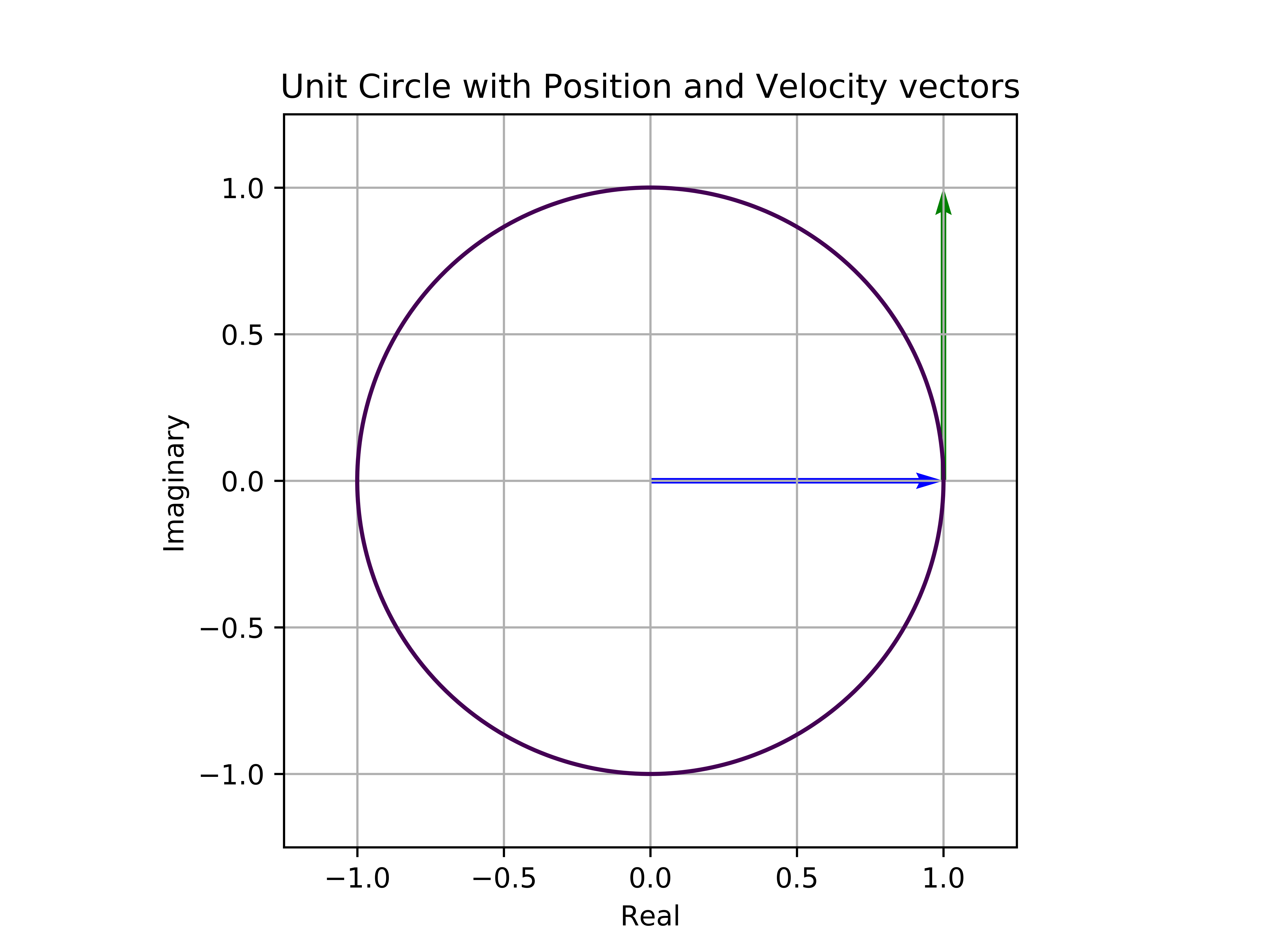
But there’s even more! Recall that the velocity vector of the trajectory is a 90-degree rotation of the position vector, i.e. \(e^{it} \perp ie^{it}\), \(\lVert e^{it} \rVert = \lVert ie^{it} \rVert\). Earlier, we concluded that the trajectory expressed by the vector \(e^{it}\) is a unit circle, which necessarily means that \(\lVert e^{it} \rVert = 1\) for all values of \(t\). Then, syllogism tells us that \(\lVert ie^{it} \rVert\) is also one, i.e. the particle on the trajectory moves at unit speed along the unit circle! Now we finally have a full visualization of the position vector.
import numpy as np
import matplotlib.pyplot as plt

x = np.linspace(-1.0, 1.0, 100)
y = np.linspace(-1.0, 1.0, 100)
x1 = np.array((0))
y1 = np.array((0))
x2 = np.array((1))
y2 = np.array((0))
vx_1 = np.array((1))
vy_1 = np.array((0))
vx_2 = np.array((0))
vy_2 = np.array((1))

X, Y = np.meshgrid(x,y)
F = X**2 + Y**2 - 1.0

fig, ax = plt.subplots()
ax.contour(X, Y, F, [0])
r = ax.quiver(x1, y1, x2, y2, units = 'xy', scale = 1, color = 'b')
v = ax.quiver(vx_1, vy_1, vx_2, vy_2, units = 'xy', scale = 1, color = 'g')
ax.set_aspect('equal')

plt.xlim(-1.25,1.25)
plt.ylim(-1.25,1.25)
plt.title('Unit Circle with Position and Velocity vectors')
plt.xlabel('Real')
plt.ylabel('Imaginary')
plt.grid(True)
plt.show()
The blue arrow represents the position vector at \(t = 0\); green, the velocity vector also at \(t = 0\).
Why is speed important? Unit speed implies that the particle moves by \(t\) distance units after \(t\) time units. Let’s say that \(\pi\) time units have passed. Where would the particle be on the trajectory now? After some thinking, we can convince ourselves that it would lie on the point \((-1, 0)\), since the unit circle has a total circumference of \(2\pi\).
And so we have proved that \(e^{i\pi} = -1\), Euler’s identity.
But we can also go a step further to derive the generalized version of Euler’s identity. Recall that a unit circle can be expressed by the following equation in the Cartesian coordinate system:
\[x^2 + y^2 = 1\]On the complex plane mapped in polar coordinates, this expression takes on an alternate form:
\[(x, yi) = (\cos t, i\sin t)\]Notice that this contains the same exact information that Euler’s identity provides for us. It expresses:
- a unit circle trajectory
- centered around the origin
- oriented counter-clockwise
- with a constant speed of 1
From this geometric interpretation, we can thus conclude that
\[e^{it} = \cos(t) + i\sin(t)\]We now know the exact value that \(e^{ix}\) represents in the complex number system!
Negative Logs, Complex Powers
Urban legend goes that mathematician Benjamin Peirce famously said the following about Euler’s identity:
Gentlemen, that is surely true, it is absolutely paradoxical; we cannot understand it, and we don’t know what it means. But we have proved it, and therefore we know it must be the truth.
But contrary to his point of view, Euler’s identity is a lot more than just an interesting, coincidental jumble of imaginary and irrational numbers that somehow churn out a nice, simple integer. In fact, it can be used to better understand fundamental operations such as logarithms and powers.
Consider, for example, the value of the following expression:
\[i^i\]Imaginary powers are difficult to comprehend by heart, and I no make no claims that I do. However, this mind-pulverizing expression starts to take more definite meaning once we consider the generalized form of Euler’s identity, \(e^{ix} = \cos(x) + i\sin(x)\).
Let \(x = \frac{\pi}{2}\). Then we have
\[e^{i\pi / 2} = \cos(\frac {\pi}{2}) + i\sin(\frac {\pi}{2}) = i\]Take both sides to the power of i:
\[{e^{i\pi / 2}}^i = e^{i^2 \pi / 2} = e^{- \pi / 2} = i^i\]Interestingly enough, we see that \(i^i\) takes on a definitive, real value. We can somewhat intuit this through Euler’s identity, which is basically telling us that there exists some inextricable relationship between real and imaginary numbers. Understood from this point of view, we see that the power operation can be defined in the entire space that is complex numbers.
We can also take logarithms of negative numbers. This can simply be shown by starting from Euler’s identity and taking the natural log on both sides.
\[e^{i \pi} = -1\] \[\ln(e^{i \pi}) = i \pi = \ln(-1)\]In fact, because \(e^{ix}\) is a periodic function around the unit circle, any odd multiple of \(\pi\) will give us the same result.
\[i(2n - 1) \pi = \ln(-1)\]While it is true that logarithmic functions are undefined for negative numbers, this proposition is only true in the context of real numbers. Once we move onto the complex plane, what may appear as unintuitive and mind-boggling operations suddenly make mathematical sense. This is precisely the magic of Euler’s identity: the marriage of different numbers throughout the number system, blending them together in such a way that seems so simple, yet so incomprehensibly complex and profound.