Relative Positional Encoding
In this post, we will take a look at relative positional encoding, as introduced in Shaw et al (2018) and refined by Huang et al (2018). This is a topic I meant to explore earlier, but only recently was I able to really force myself to dive into this concept as I started reading about music generation with NLP language models. This is a separate topic for another post of its own, so let’s not get distracted.
Let’s dive right into it!
Concept
If you’re already familiar with transformers, you probably know that transformers process inputs in parallel at once. This is one of the many reasons why transformers have been immensely more successful than RNNs: RNNs are unable to factor in long-range dependencies due to their recurrent structure, whereas transformers do not have this problem since they can see the entire sequence as it is being processed. However, this also means that transformers require positional encodings to inform the model about where specific tokens are located in the context of a full sequence. Otherwise, transformer would be entirely invariant to sequential information, considering “John likes cats” and “Cats like John” as identical. Hence, positional encodings are used to signal the absolute position of each token.
Relative Positional Encoding
While absolute positional encodings work reasonably well, there have also been efforts to exploit pairwise, relative positional information. In Self-Attention with Relative Position Representations, Shaw et al. introduced a way of using pairwise distances as a way of creating positional encodings.
There are a number of reasons why we might want to use relative positional encodings instead of absolute ones. First, using absolute positional information necessarily means that there is a limit to the number of tokens a model can process. Say a language model can only encode up to 1024 positions. This necessarily means that any sequence longer than 1024 tokens cannot be processed by the model. Using relative pairwise distances can more gracefully solve this problem, though not without limitations. Relative positional encodings can generalize to sequences of unseen lengths, since theoretically the only information it encodes is the relative pairwise distance between two tokens.
Relative positional information is supplied to the model on two levels: values and keys. This becomes apparent in the two modified self-attention equations shown below. First, relative positional information is supplied to the model as an additional component to the keys.
\[e_{ij} = \frac{x_i W^Q (x_j W^K + a_{ij}^K)^\top}{\sqrt{d_z}} \tag{1}\]The softmax operation remains unchanged from vanilla self-attention.
\[\alpha_{ij} = \frac{\text{exp} \space e_{ij}}{\sum_{k = 1}^n \text{exp} \space e_{ik}}\]Lastly, relative positional information is supplied again as a sub-component of the values matrix.
\[z_i = \sum_{j = 1}^n \alpha_{ij} (x_j W^V + a_{ij}^V) \tag{2}\]In other words, instead of simply combining semantic embeddings with absolute positional ones, relative positional information is added to keys and values on the fly during attention calculation.
Bridging Shaw and Huang
In Huang et al., also known as the music transformer paper, the authors pointed out that calculating relative positional encodings as introduced in Shaw et al. requires $O(L^2D)$ memory due to the introduction of an additional relative positional encoding matrix. Here, $L$ denotes the length of the sequence, and $D$, the hidden state dimension used by the model. Huang et al. introduced a new way of computing relative positional encoding via a clever skewing operation.
To cut to the chase, below is the relative attention mechanism suggested by the authors in Huang et al.
\[\text{RelativeAttention} = \text{Softmax} \left( \frac{Q K^\top + S_{rel}}{\sqrt{D_h}} \right) V \tag{3}\]It seems that in the music transformer paper, the authors dropped the additional relative positional embedding that corresponds to the value term and focus only on the key component. In other words, the authors only focus on (1), not (2).
The notations in (1), (2), and (3) were each borrowed verbatim from the authors of both papers. Hence, there is some notational mixup that requires attention. Specifically, $S^{rel}$ in the music transformer paper is simply
\[S_{rel} = Q R^\top\]where
\[R_{ij} = a_{ij}^K\]In other words, (3) is just an expanded variant of (1).
To make things a little clearer, let’s review the dimensions of each tensor. First, from vanilla self-attention, we know that $Q \in \mathbb{R}^{H \times L \times D_h}$, where $H$ denotes the number of heads. Thus, $R \in \mathbb{R}^{H \times L \times D_h}$, and $S_{rel} \in \mathbb{R}^{H \times L \times L}$. $R$ is a matrix of relative positional embeddings. Intuitively, $R$ can also be understood as the result of passing a matrix of relative positional indices through an embedding layer. For concreteness, here is a dummy function that creates relative positional indices.
Efficient Computation
The skewing mechanism introduced in Huang et al., is ingenious, but it isn’t black magic. The technique could roughly be understood as a set of clever padding and matrix manipulation operations that ultimately result in $S_{rel}$ without explicitly creating or computing $R$. The reason why we might want to avoid calculating $R$ is that it is a huge memory bottleneck, as the matrix requires $O(L^2 d)$ extra space.
The method presented by Huang et al. could be seen as follows:
def relative_positions(seq_len):
    result = []
    for i in range(seq_len):
        front = list(range(-i, 0))
        end = list(range(seq_len - i))
        result.append(front + end)
    return result
Let’s see what the indices look like for a sequence of length five.
relative_positions(5)
[[0, 1, 2, 3, 4],
 [-1, 0, 1, 2, 3],
 [-2, -1, 0, 1, 2],
 [-3, -2, -1, 0, 1],
 [-4, -3, -2, -1, 0]]
We can understand each row as indicating the current position of attention, and each index as representing the distance between the current token and the token corresponding to the index. A quick disclaimer that this example does not strictly follow the details outlined in Shaw et al. For instance, this function does not take into account $k$, or the width of the window. The 0-based indexing scheme is also from Huang et al. These minor details notwithstanding, having a clear sense of what $R$ is, I think, is very helpful in understanding relative attention, as well as the skewing mechanism introduced in Huang et al. For a fuller explanation of these concepts, I highly recommend this medium article.
Below is a visual summary of the skewing mechanism.
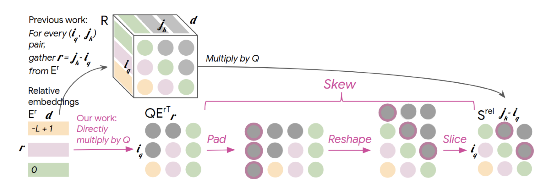
Personally, I found this diagram to be a bit confusing at first. However, with must staring and imagination, I slowly started to realize that the skewing is simply a way of transforming $QE_r^\top$ into $QR^\top$, where $E_r$ is the relative positional embedding matrix.
Instead of trying to explain this in plain text, I decided that implementing the the entire relative global attention would not only help with demonstration, but also cementing my own understanding of how this works.
Implementation
This implementation of relative global attention was in large part influenced by Karpathy’s minGPT, which we discussed in this previous post, as well as Prayag Chatha’s implementation of the music transformer, available on GitHub here.
import math
import torch
from torch import nn
import torch.nn.functional as F
Below is a simple implementation of a relative global attention layer. I’ve deviated from Chatha’s implementation in a number of ways, but the most important and probably worth mentioning is how I treat the relative positional embedding matrix. In Shaw et al., the authors note that “[relative positional embeddings] can be shared across attention heads.” Hence, I’m using one Er matrix to handle all heads, instead of creating multiple of them. This matrix is registered as a nn.Parameter.
class RelativeGlobalAttention(nn.Module):
    def __init__(self, d_model, num_heads, max_len=1024, dropout=0.1):
        super().__init__()
        d_head, remainder = divmod(d_model, num_heads)
        if remainder:
            raise ValueError(
                "incompatible `d_model` and `num_heads`"
            )
        self.max_len = max_len
        self.d_model = d_model
        self.num_heads = num_heads
        self.key = nn.Linear(d_model, d_model)
        self.value = nn.Linear(d_model, d_model)
        self.query = nn.Linear(d_model, d_model)
        self.dropout = nn.Dropout(dropout)
        self.Er = nn.Parameter(torch.randn(max_len, d_head))
        self.register_buffer(
            "mask",
            torch.tril(torch.ones(max_len, max_len))
            .unsqueeze(0).unsqueeze(0)
        )
        # self.mask.shape = (1, 1, max_len, max_len)


    def forward(self, x):
        # x.shape == (batch_size, seq_len, d_model)
        batch_size, seq_len, _ = x.shape

        if seq_len > self.max_len:
            raise ValueError(
                "sequence length exceeds model capacity"
            )

        k_t = self.key(x).reshape(batch_size, seq_len, self.num_heads, -1).permute(0, 2, 3, 1)
        # k_t.shape = (batch_size, num_heads, d_head, seq_len)
        v = self.value(x).reshape(batch_size, seq_len, self.num_heads, -1).transpose(1, 2)
        q = self.query(x).reshape(batch_size, seq_len, self.num_heads, -1).transpose(1, 2)
        # shape = (batch_size, num_heads, seq_len, d_head)

        start = self.max_len - seq_len
        Er_t = self.Er[start:, :].transpose(0, 1)
        # Er_t.shape = (d_head, seq_len)
        QEr = torch.matmul(q, Er_t)
        # QEr.shape = (batch_size, num_heads, seq_len, seq_len)
        Srel = self.skew(QEr)
        # Srel.shape = (batch_size, num_heads, seq_len, seq_len)

        QK_t = torch.matmul(q, k_t)
        # QK_t.shape = (batch_size, num_heads, seq_len, seq_len)
        attn = (QK_t + Srel) / math.sqrt(q.size(-1))
        mask = self.mask[:, :, :seq_len, :seq_len]
        # mask.shape = (1, 1, seq_len, seq_len)
        attn = attn.masked_fill(mask == 0, float("-inf"))
        # attn.shape = (batch_size, num_heads, seq_len, seq_len)
        attn = F.softmax(attn, dim=-1)
        out = torch.matmul(attn, v)
        # out.shape = (batch_size, num_heads, seq_len, d_head)
        out = out.transpose(1, 2)
        # out.shape == (batch_size, seq_len, num_heads, d_head)
        out = out.reshape(batch_size, seq_len, -1)
        # out.shape == (batch_size, seq_len, d_model)
        return self.dropout(out)


    def skew(self, QEr):
        # QEr.shape = (batch_size, num_heads, seq_len, seq_len)
        padded = F.pad(QEr, (1, 0))
        # padded.shape = (batch_size, num_heads, seq_len, 1 + seq_len)
        batch_size, num_heads, num_rows, num_cols = padded.shape
        reshaped = padded.reshape(batch_size, num_heads, num_cols, num_rows)
        # reshaped.size = (batch_size, num_heads, 1 + seq_len, seq_len)
        Srel = reshaped[:, :, 1:, :]
        # Srel.shape = (batch_size, num_heads, seq_len, seq_len)
        return Srel
Much of the operations in forward method are code translations of the equations we discussed above. The interesting bit happens in the skew method. Basically, we pad $Q E_r^\top$ to the left, then reshape to shift all indices, then slice out the necessary portion of the matrix to obtain $Q R^\top$, or $S_{rel}$. This has the benefit of reducing the memory requirement; since we don’t have to calculate $R$ and can instead directly use $E_r$, which is a matrix that is needed anyway, the memory requirement is reduced to $O(Ld)$. This is what I personally think is one of the biggest contributions of Huang et al.
Let’s quickly check that the layer works as intended by quickly performing a basic tensor shape check.
batch_size = 8
seq_len = 100
d_model = 768
num_heads = 12

test_in = torch.randn(batch_size, seq_len, d_model)
l = RelativeGlobalAttention(d_model, num_heads)
l(test_in).shape
torch.Size([8, 100, 768])
We get an output of size (batch_size, seq_len, d_model), which is what we expect.
Conclusion
In this post, we discussed relative positional encoding as introduced in Shaw et al., and saw how Huang et al. was able to improve this algorithm by introducing optimizations.
Relative positional encodings were used in other architectures, such as Transformer XL, and more recently, DeBERTa, which I also plan on reviewing soon. Relative positioning is probably a lot closer to how we humans read text. While it is probably not a good idea to always compare and conflate model architectures with how the human brain works, I still think it’s an interesting way to think about these concepts.
This post was also a healthy exercise in that it really forced me to try to understand every single detail. Every sentence and diagram can be of huge help when you are trying to actually implement ideas that are outlined in published papers. I could see why Papers with Code became such a huge thing. It’s always helpful to see actual implementations and, even better, reproducible results. In this particular post, referencing music transformer implementations on GitHub and re-reading the paper many times really helped me nail down points that were initially confusing or unclear.
I hope you’ve enjoyed reading this post. Catch you up in the next one!