Locality Sensitive Hashing

These days, I’ve found myself absorbed in the world of memory-efficient transformer architectures. Transformer models require $O(n^2)$ runtime and memory due to how self-attention is implemented. Namely, each token has to be attended with every other token in the sequence, and the results must be stored in a square attention matrix, to which we apply a softmax activation to obtain the weights to multiply the values with.

So far, many researchers have presented various ways of optimizing this computation while decreasing the algorithm down to linear runtime. Such architectures include the Linformer, Reformer, Performer, LongFormer, and more recently, the Nyströmformer. My knowledge base is way too shallow to be able to read these papers on my own. Thankfully, there are heros like Yannic Kilcher who help make trendy deep learning papers a lot more accessible, even for novices like myself. I cannot recommend his channel enough.

Today, we’ll explore an algorithm known as LSH, or locality-sensitive hashing. LSH was used in Reformer, which is one of the linear-runtime transformer models in the list. This is intended as a beginner-friendly introduction to this topic; I hope other readers can get a sense of what it is and have a better time understanding how the Reformer architecture works. As supplements, I also suggest that you check out this medium article as well as this blog post, both of which I referenced in writing this post.

Without further ado, let’s get started!

Concept

Imagine that you are building a music identification service like Shazam. You probably have a huge database of songs. Whenever a user plays a song, the engine should be able to conduct some sort of scan through the database to find which row best matches the song that is being played by the user. We can imagine, for instance, that the entire database is a matrix, and that each song is a vectorized row. We would some kind of distance metric, like cosine similarity, to determine how well a given song matches the user query.

If we have a relatively small database, a linear scan could work. However, when there are millions and billions of songs, perhaps that’s not the best implementation. If each song is encoded as a high-dimensional vector, perhaps a multiplication involving trillion-by-million matrix is not really tractable in computational terms. One thing we could do to remedy this is to use a dimensionality reduction technique, like PCA. We can also try to do some clustering or bucketing.

LSH is an algorithm that can accomplish both tasks at once: namely, dimensionality reduction via hasing, and clustering of sorts via bucketing or binning. Let’s walk through this process step-by-step.

Hashing

There are many ways of hashing. So far, I’ve looked at two examples, which are min-hashing (also known as min-wise independent permutations) and random projections. In this post, we will look at the random projection method, which not only do I find intuitive, but also is the method that was used in the Reformer paper.

In most contexts, the goal of hashing is to map some item to a unique point living in another space. In other words, if $a \neq b$, then we hope that

\[h(a) \neq h(b)\]

where $h()$ is a hashing function.

In the context of LSH, however, this is not the case. In fact, we want similar data points to be mapped to the same point, with high probability. In other words, given some large threshold value $0 \leq \alpha \leq 1$, we want

\[\text{Pr}(h(a) = h(\tilde{a})) \geq \alpha\]

where $\tilde{a}$ denotes a data point that is similar or close to $a$. In LSH-specific terms, we want the two data points to end up in the same bucket after going through the hash function. Going back to our music identification example, we could think of LSH as clustering similar songs into the same category.

Projection

While there are many different hash functions we could use for the purposes of LSH (note that cryptographic hashing functions such as SHA will not work here for the reason mentioned above), for our purposes, we will be taking a look at random projections.

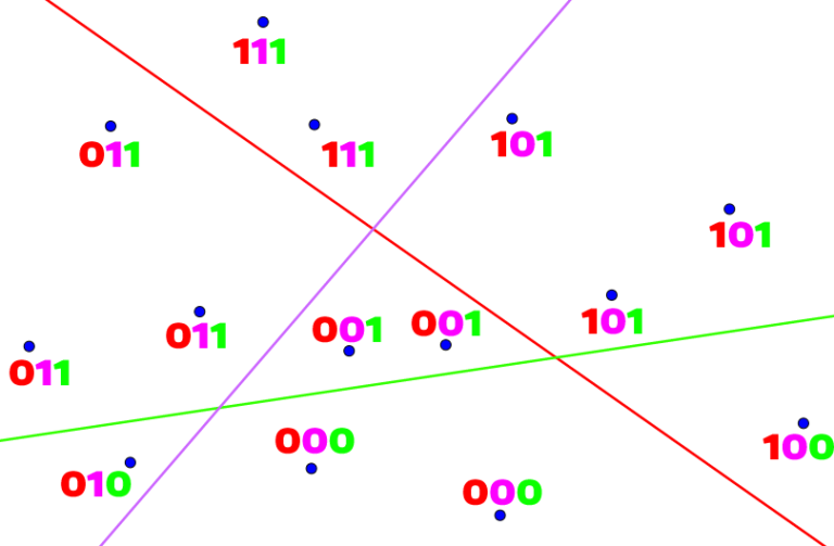
The intuition behind random projections are simple: given high-dimensional data points, we want to project these vectors down to lower dimensions where similar vectors will be grouped together into the same bucket. More concretely, we can come up with $k$ random vectors, and project each data point to each of these vectors. If, for example, the dot product between the $i$th random vector and a data point is positive, then we encode that information by having the $i$th index of the resulting hashed representation as 1; if it is zero or a negative value, we denote it as 0. At the end of the day, each data point would thus be mapped to a binary vector of length $k$. Below is an illustration taken fro Code Forces that better visualizes this concept.

The resulting binary vectors are then put into buckets. The number of buckets will be at most $2^k$, since this is the total number of representations that are possible given a $k$-dimensional binary vector. In the illustration above, $k=3$, and each binary vector becomes a bucket of its own.

Implementation

All of this could have sounded a little abstract and confusing, but in reality, it’s really nothing more than just matrix multiplication.

Let’s first import NumPy.

import numpy as np

init_dim refers to the original dimension in which our high-dimensional data points are living. num_data is the total number of data points. From these pieces of information, we can deduce that the design matrix $D \in \mathbb{R}^{10 \times 5}$. Last but not least, num_rvecs denotes the number of random vectors. To make things simple, we set it to a small number.

init_dim = 5
num_data = 10
num_rvecs = 2

The number of random vectors is what will determine the number of buckets. Intuitively, it is not difficult to see that, the higher the number of random vectors, the more fine grained the final binary outputs will be. This also means, however, that every bucket will probably end up having only a few data points each, which defeats the purpose of bucketting via LSH.

Let’s create a contrieved dataset.

data = np.random.randn(num_data, init_dim)
data.shape

(10, 5)

Next, let’s create a matrix containing random vectors. This can loosely be referred to as the projection matrix.

proj = np.random.randn(init_dim, num_rvecs)
proj

array([[ 1.3013903 , -2.34361703],
       [ 0.14915403, -1.0453711 ],
       [-0.47002247, -0.16004093],
       [ 1.30216575, -0.49852838],
       [ 0.06249788,  0.19392549]])

Note that each column is a random vector. This could be somewhat confusing, as we are used to seeing each row as a distinct item, but for matrix multiplication purposes, consider this a transposed matrix.

Now, we can obtain the result of the projection by simply computing the product of the two matrices.

result = data @ proj
result

array([[-0.47585172,  2.05332923],
       [ 0.36156221, -1.89596521],
       [-2.61458497,  2.98516562],
       [ 1.2037197 , -0.36646877],
       [ 2.33599015, -4.88713399],
       [ 0.80701667, -2.19645812],
       [-2.01608837,  1.98033745],
       [-0.06135221,  0.27154208],
       [ 0.28265284, -0.23497936],
       [-0.14683807,  0.75087065]])

Notice that the ten data points, which were previously 15-dimensional, have now been projected down to three dimensions. But still, we can’t perform bucketting quite yet; to finalize hashing via random projections, we need to encode this result as binary vectors. This can simply done by comparing the matrix with 0.

hashed = list(map(tuple, (result > 0).astype(int)))
hashed

[(0, 1),
 (1, 0),
 (0, 1),
 (1, 0),
 (1, 0),
 (1, 0),
 (0, 1),
 (0, 1),
 (1, 0),
 (0, 1)]

And voila! We now have binary, hashed representations for each data point. Let’s take a closer look. Notice that the first and third data points have all ended up as (0, 1). This means that (0, 1) forms a bucket containing the first two data points. The same goes for other data points: those with identical binary representations belong in one bucket.

We can systematically do perform this bucketting with the following code snippet.

from collections import defaultdict

buckets = defaultdict(list)

for i, row in enumerate(hashed):
    buckets[row].append(i)

And we see that there are a total of 5 buckets.

dict(buckets)

{(0, 1): [0, 2, 6, 7, 9], (1, 0): [1, 3, 4, 5, 8]}

A good LSH algorithm implementation would most likely ensure that every bucket has roughly the same amount of data points. Moreover, the buckets would reflect actual distances between data points in their original dimension. In other words, data points that were close to each other would probably end up in the same bucket. The randomness of the projection tries to ensure this property.

first_row = data[0]

distances = np.array([np.dot(row, first_row) for row in data])
np.argsort(distances)

array([4, 5, 3, 8, 2, 1, 9, 7, 6, 0])

It appears that 4, 5, 3, 8, and 2 are data points that are far away from the first (or zero-indexed) data point. Our toy LSH implementation almost got them correct, with the exception of placing 2 in the same bucket instead of 1. However, given that 2 and 1 were right next to each other, perhaps the algorithm has done reasonably well here in binning vectors by their distance in their original high-dimensional space.

Conclusion

Locality sensitive hashing can be used in many places. The music identification engine is an obvious one, where we would basically hash songs in the database into buckets. Then, we would perform the same hashing on the user input, see which bucket it lands on, and only query those candidates within the same bucket. This greatly reduces the number of linear scanning that has to take place.

In the context of the transformer architecture, researchers who developed Reformer reduced the number of computations needed to produce the attention matrix, by basically binning the key and query vectors into appropriate buckets, and performing self-attention only within those buckets. This exploits the fact that the weighted value vector only largely depends on keys with high attention coefficients, since the softmax tends to squash lesser values and augments larger ones. This is a very cursory explanation of how the Reformer optimizes attention calculation; we will probably explore this in a separate blog post.

I hope you’ve enjoyed reading this article. Catch you up in the next one!