R Tutorial (2)

In this post, we will continue our journey with the R programming language. In the last post, we explored some basic plotting functions and how to use them to visualize data. In this post, we will take a break from commands relating to visualization and instead focus on some tools for statistical analysis on distributions. Let’s jump right in.

Binomial Distribution

Let’s consider the simple example of a fair coin toss, just because we are uncreative and like to recycle overused examples in textbooks.

\[X \sim \text{Binom}(n=20, p=0.5)\]

The dbinom function is used to calculate the probability desntiy function (or the probability mass function in the discrete case). For example, we might compute $P(X = 10)$ as follows:

dbinom(x=10, size=20, prob=0.5)

## [1] 0.1761971

We can also use slicing to obtain $p(0) + p(1) + ⋯ + p(10)$, if that quantity is ever an interest to us.

sum(dbinom(x=0:10, size=20, prob=0.5))

## [1] 0.5880985

Notice that the sum function was used in order to aggregate all the values in the returned list. As you can see, this is one way one might go about calculating the cumulative mass function. CDFs cannot be computed in this fashion since slicing of integers from 0:10 cannot be used for continuous random variables.

There is a more direct way to calculate the CMF right away without using the sum command, and that is pbinom. Here is a simple demonstration.

pbinom(q=10, size=20, prob=0.5, lower.tail=TRUE)

## [1] 0.5880985

As expected we get the same exact value. The lower.tail argument tells R that we want values lesser or equal to 10, inclusive.

Quite similarly, we can also use qbinom as a quantile function, which can be considered as the inverse of pbinom in the sense that it gives us a q value instead of a p value.

qbinom(p=0.5880985, size=20, prob=0.5)

## [1] 10

The dbinom and pbinom commands we have looked so far dealt with probability mass functions of the binomial distribution. But what if we want to sample a random variable from this distribution, say to perform some sort of Monte Carlo approximation? This can be achieved with the rbinom command.

rbinom(n=5, size=20, prob=0.5)

## [1] 10  6  8 10  7

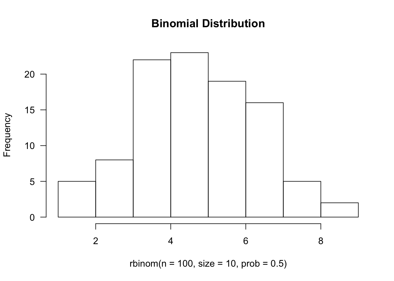
Note that this is a simulation of the binomial random variable, not Bernoulli. Since we specified n=5, we get five numbers. If we repeat this many times, it turns into a very primitive form of Monte Carlo simulation.

hist(rbinom(n=100, size=10, prob=0.5), main='Binomial Distribution', las=1)

Normal Distribution

One useful pattern to realize is that the designers of R were very systematic: they didn’t name functions out of arbitrary whim. Instead, there is a set pattern, where it strictly adheres to the form *{dist}, where * is a single character, one of d, p, q, or r. Here is a quick rundown of what each of these characters signify:

• d: PDF or PMF
• p: CDF or CMF
• q: Inverse CDF or CMF
• r: Random sampling from distribution

Given this piece of information, perhaps it’s unsurprising that the commands for the normal distribution are dnorm, pnorm, qnorm, and rnorm. Let’s start with the first one on the list, dnorm.

dnorm(x=0, mean=0, sd=1)

## [1] 0.3989423

Recall that the equation for a univariate standard normal distribution is given by

\[p(x) = \frac{1}{\sqrt{2 \pi}} e^{- \frac{x^2}{2}}\]

If you plug in x = 0 into this equation, you will see (perhaps with the help of Wolfram) that the value returned by the function, which is simply the normalizing constant, is indeed approximately 0.39. In short, dnorm represents the PDF of the normal distribution.

The next on the list is pnorm, which we already know models the Gaussian CDF. This can easily be verified by the fact that

pnorm(q=0, mean=0, sd=1)

## [1] 0.5

This is expected behavior, since q=0 corresponds to the exact mid-point of the Gaussian PDF.

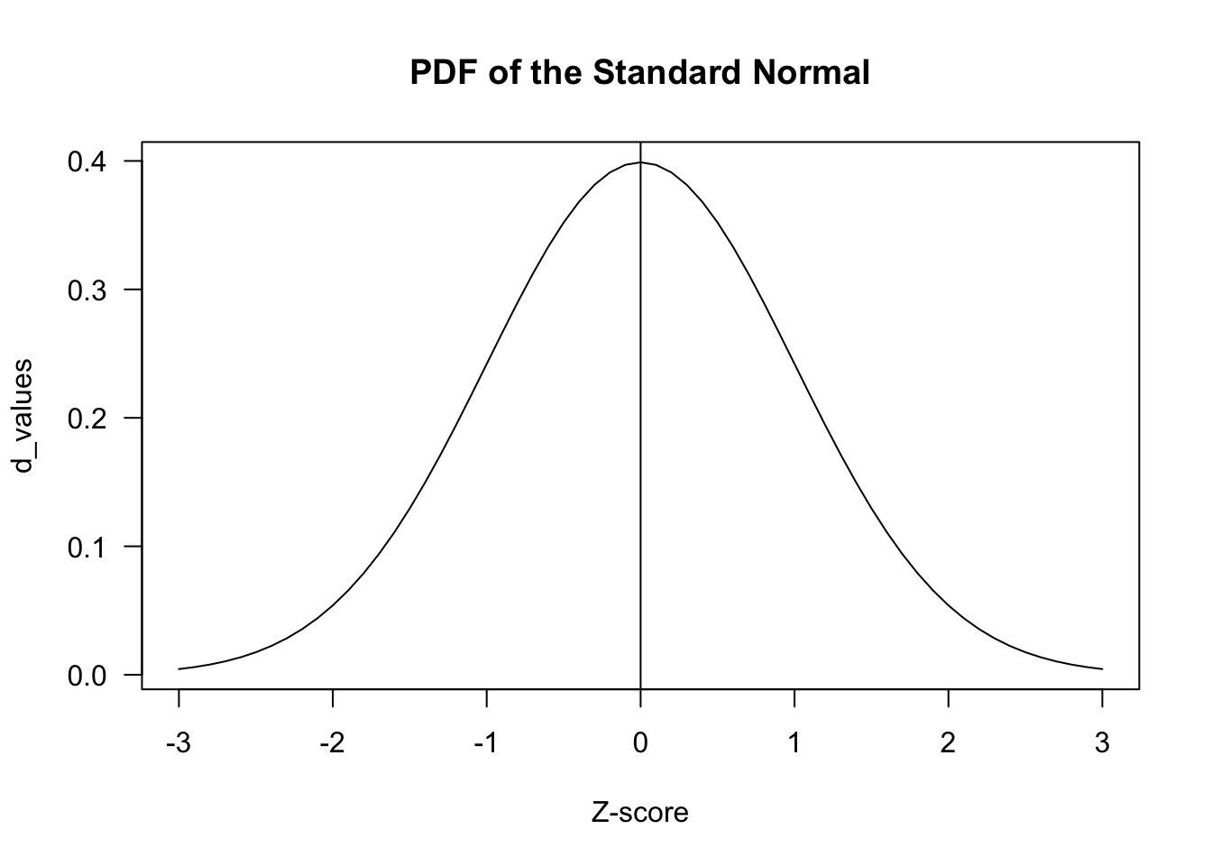
z_scores <- seq(-3, 3, by = .1)
d_values <- dnorm(z_scores)
plot(z_scores, d_values, type="l", main = "PDF of the Standard Normal", xlab= "Z-score", las=1)
abline(v=0)

As a bite-sized exercise, let’s try to take a look at the empirical rule of the Normal distribution, namely that values within one standard deviation from the mean cover roughly 68% of the entire distribution.

pnorm(q=1, mean=0, sd=1) - pnorm(q=-1, mean=0, sd=1)

## [1] 0.6826895

We could have also used the lower.tail argument, which defines in which direction we calcalate the CDF. If lower.tail is set to FALSE, then the function returns the integral from q to infinity of the PDF of the normal distribution.

1 - pnorm(q=-1, mean=0, sd=1) - pnorm(q=1, mean=0, sd=1, lower.tail=FALSE)

## [1] 0.6826895

The qnorm is best understood as the inverse CDF function. This means that the function would receive as input the value of the area under the function, which can also be interpreted as the $z$-score.

qnorm(p=0.5, mean=0, sd=1)

## [1] 0

We can directly verify the fact that qnorm is an inverse of pnorm by pluggin in a value.

pnorm(qnorm(1))

## [1] 1

Last but not least, the rnorm function can be used to sample values from the normal distribution with the specified parameters. Let’s start by sampling 10 values from the standard normal distribution.

rnorm(10, mean=0, sd=1)

##  [1]  1.4539733  0.7706782 -0.2794539 -0.9202353 -0.1092644 -0.2717883
##  [7] -0.9901838  0.7300424  0.9494669 -0.9996891

We can also set the seed to make sure that results are replicable. The command does not return anything; it merely sets the seed for the current thread.

set.seed(42)

Poisson Distribution

Recall that a Poisson distribution is used to model the probability of having some number of events occuring within a window of unit time given some rate parameter λ. Suppose that the phenomenon we’re modeling has an average rate of 7. If we want to know the probability $P(X = 5)$, we can use the dpois function to calculate the PMF:

lambda <- 7
dpois(x=5, lambda=lambda)

## [1] 0.1277167

Therefore, we know that there is a 0.127 probability of exactly five occurences.

Because R is by nature a vectorized language, we can also pass into the x argument a sequence of numbers, the result of which would also be a sequence. We saw this technique earlier with dbinom, but let’s just try it again for the sake of explicitness. For example,

x <- seq(1, 14)
dpois(x=x, lambda=lambda)

##  [1] 0.006383174 0.022341108 0.052129252 0.091226192 0.127716668
##  [6] 0.149002780 0.149002780 0.130377432 0.101404670 0.070983269
## [11] 0.045171171 0.026349850 0.014188381 0.007094190

From here, we can move onto discussing ppois, the CMF, or qpois, the inverse CMF, and rpois, the random sampling function, but going over them one by one would be a mere repetition of what we’ve done so far with the binomial and the normal. Therefore, let’s try something different. Namely, let’s try to empirically verify the Central Limit Theorem (CLT), using various R distribution and sampling functions we have looked at so far.

Re call that CLT stipulates that, as the number of samples n goes to infinity,

\[\sqrt{n}\left(\frac{\bar{X\_n} - \mu}{\sigma} \right) \sim \mathcal{N}(0, 1)\]

where

\[\bar{X_n} = \frac1n(X_1 + X_2 + \cdots + X_n)\]

This is basically a specification of the Law of Large Numbers, which simply states that the sample mean converges to the true mean as n goes to infinity. CLT goes a step beyond LLN, stating that the distribution approximates a Gaussian.

While we won’t be mathematically proving CLT or LLN, we can instead try to see if random sampling supports their stipulations by setting a value for n that is reasonably large enough for estimation purposes.

n <- 1000
rows <- 1000
sim <- rpois(n=n*rows, lambda=lambda)

sim is going to be a vector of 100000 integers, each number representing a random sample from the Poisson distribution. What we need to do, now, is to calculate the sample mean, where n equals 100. To achieve this, we will reshape sim into a matrix, then calculate the mean of each row.

mat <- matrix(data=sim, nrow=rows)
sample.means <- apply(X=mat, MARGIN=1, FUN=mean)

Let’s plot sample.mean to first see if this indeed looks like a Gaussian.

hist(sample.means)

!

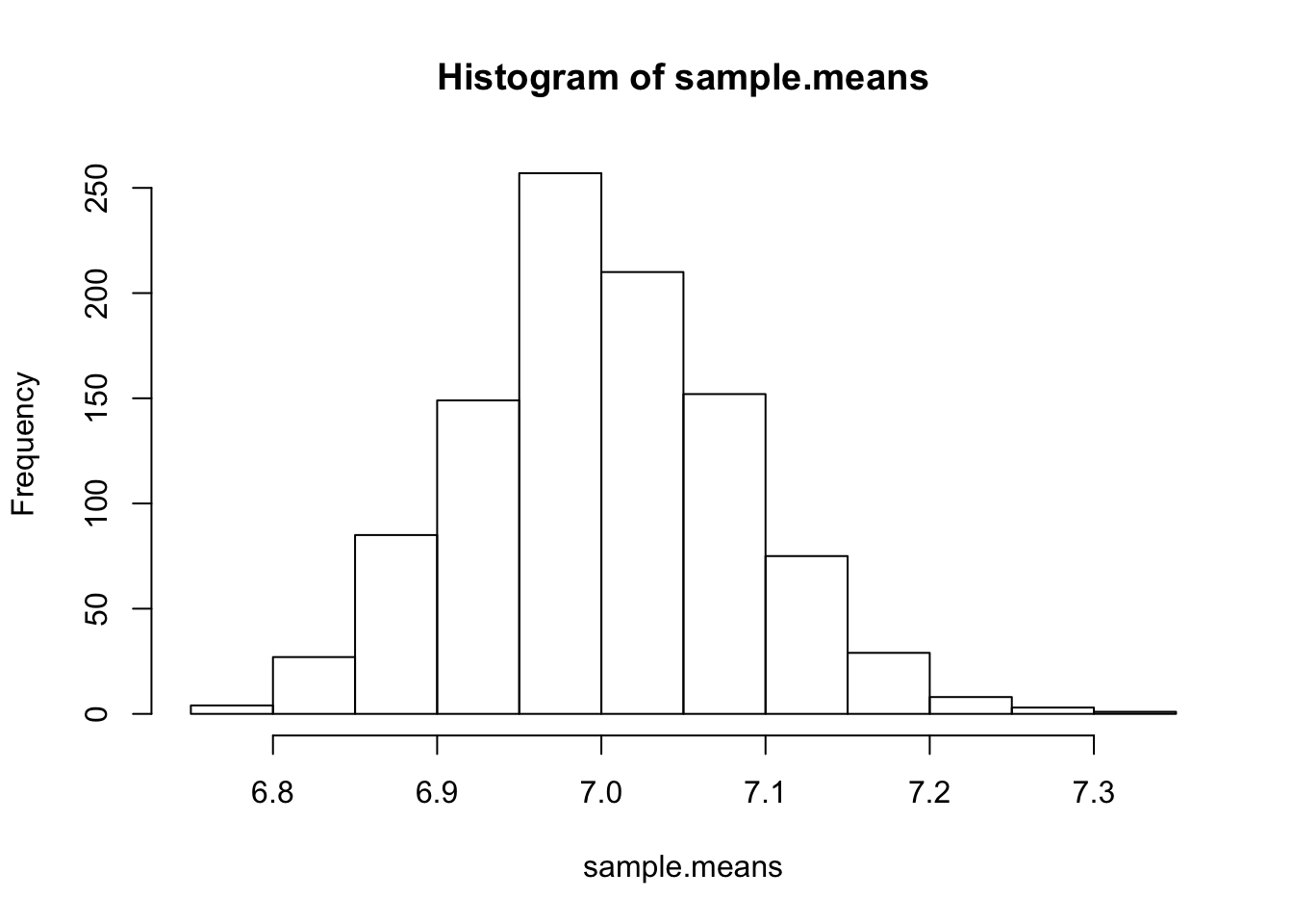
It’s certainly not exactly a Gaussian, but at least it does not unimodal and symmetric. If LLN and CLT is true, then we already know the mean and variance of this normal distribution: the mean is simply the rate parameter, 7, and the variance can be calculated as \(\begin{align} \text{Var}[\bar{X_n}] &= \text{Var}\left[\frac{1}{n}(X_1 + X_2 + \cdots + X_n) \right] \\ &= \frac{1}{n^2}(\text{Var}[X_1] + \text{Var}[X_2] + \cdots + \text{Var}[X_n]) \\ &= \frac{\text{Var}[X]}{n} \\ &= \frac{\lambda}{n} \tag{1} \end{align}\)

Let’s see if these are indeed true. First, we can verify the mean of the sample means via

mean(sample.means)

## [1] 6.999988

That is sure enough close to 7, as we would expect. Then, there’s variance:

sd(sample.means)^2

## [1] 0.006953299

lambda/n

## [1] 0.007

And indeed, it seems like the results match. Note that the second calculation is based on the results in (1). Note that in specifying dnorm, we didn’t have to specify a range by creating a seq or using : slicing; instead, R is able to understand that x is a variable.

hist(sample.means, breaks=20, freq=F)
curve(dnorm(x, mean=7, sd=sqrt(0.007)), add=T)

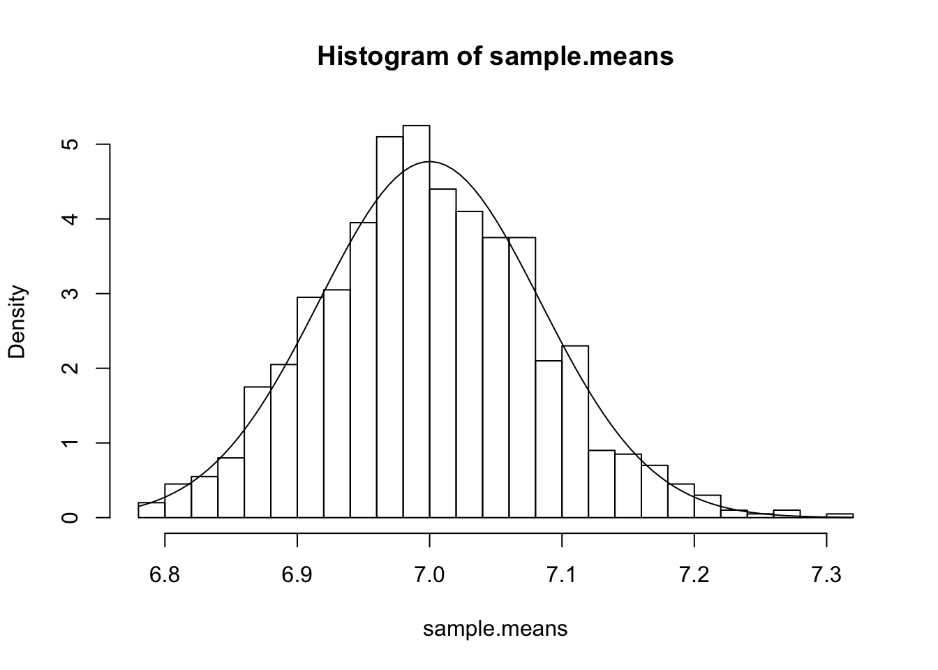
The result seems to quite strongly vindicate CLT and LLN, as expected.

Conclusion

Today’s post introduced some very useful functions relating to probability distributions. The more I dive into R, the more I’m amazed by how powerful R is as a statistical computing language. While I’m still trying to wrap my head around some of R’s quirky syntax (as a die-hard Pythonista, I think Python’s syntax is more intuitive), but this minor foible is quickly offset by the fact that it offers powerful vectorization, simulating, and sampling features. I love NumPy, but R just seems to do a bit better in some respects.

In the next post, we will be taking a look at things like the t-distribution and hypothesis testing. Stay tuned for more!