Understanding PageRank

Google is the most popular search engine in the world. It is so popular that the word “Google” has been added to the Oxford English Dictionary as a proper verb, denoting the act of searching on Google.

While Google’s success as an Internet search engine might be attributed to a plethora of factors, the company’s famous PageRank algorithm is undoubtedly a contributing factor behind the stage. The PageRank algorithm is a method by which Google ranks different pages on the world wide web, displaying the most relevant and important pages on the top of the search result when a user inputs an entry. Simply put, PageRank determines which websites are most likely to contain the information the user is looking for and returns the most optimal search result.

Network Graph Representation

While the nuts and bolts of this algorithm may appear complicated—and indeed they are—the underlying concept is surprisingly intuitive: the relevance or importance of a page is determined by the number of hyperlinks going to and from the website. Let’s hash out this proposition by creating a miniature version of the Internet. In our microcosm, there are only five websites, represented as nodes on a network graph. Below is a simple representation created using Python and the Networkx package.

import networkx as nx
import matplotlib.pyplot as plt

# Initialize a directed graph
DG = nx.DiGraph()

# Create a list of webpages
pages = ["A", "B", "C", "D", "E"]

# Add nodes
DG.add_nodes_from(pages)

# Create a list of hyperlinks
# (X, Y) represents a directed edge from X to Y
links = [
("A", "B"), ("B", "A"), 
("B", "C"), ("C", "A"), 
("C", "B"), ("C", "E"), 
("D", "A"), ("E", "D"), 
("E", "B"), ("E", "C")
]

# Add edges
DG.add_edges_from(links)

# Draw graph
nx.draw(DG, with_labels = True)
plt.draw()
plt.show()

Running this block results in the following graph:

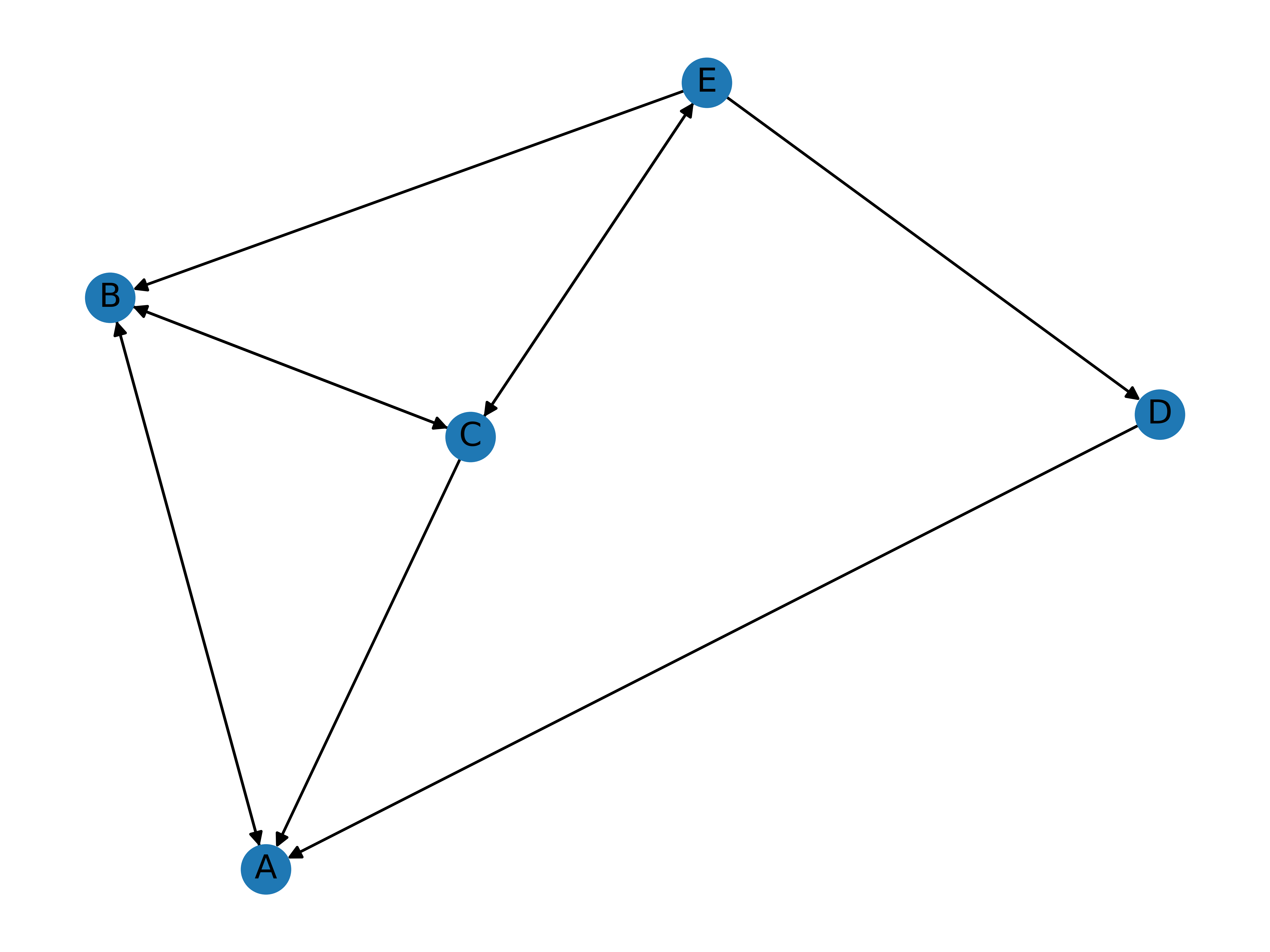
How is this a model of the Internet? Well, as simple as it seems, the network graph contains all the pertinent information necessary for our preliminary analysis: namely, hyperlinks going from one page to another. Let’s take node D as an example. The pointed edges indicate that page E contains a link to page D, and that page D contains another link that redirects the user to page A. Interpreted in this fashion, the graph indicates which pages have a lot of incoming and outgoing reference links.

But all this aside, why are hyperlinks important for the PageRank algorithm in the first place? A useful intuition might be that websites with a lot of incoming references are likely to be influential sources, often written by prominent individuals. This analysis is certainly the case in the field of academics, where works of literature that are frequently cited quickly gain clout and attain an established position in the given discipline. Another reasoning is that hyperlinks tell us where a user is most likely to wound up in after browsing through returned search results. Take the extreme example of an isolated node, where there are zero outgoing and ingoing links to the website. It is unlikely that a user will end up on that webpage, as opposed to a popular site with a spiderweb of edges on a network graph. Then, it would make sense for the PageRank algorithm to display that website on top; the isolated node, the bottom.

Markov Chain

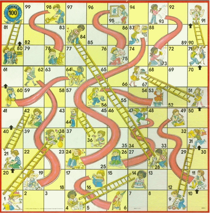
Suppose we want to know where a user is most likely to end up in after a given search. This process is often referred to as a random walk because, as the name suggests, it describes a path after a succession of random steps on some mathematical space. While it is highly unlikely that a user visits a website, randomly selects one of the hyperlinks on the given page, and repeats the two steps above repeatedly, the assumption on randomness is what allows us to simulate a user’s navigation of the Internet from the point of view of Markov chains, a stochastic model that describes a sequence of possible events, or states, in which the probability of each event is contingent only upon the previous state attained in the previous event. One good example of a Markov chain is the famous Chutes and Ladders game, in which the player’s next position is dependent only upon their present position on the game board. For this reason, Markov chains are said to be memoryless: in the Chutes and Ladders game, whether the player ended up in their current position by taking a ladder or a normal dice roll is irrelevant to the progress of the game.

A salient characteristic of a Markov chain is that the probabilities of each event can be represented and calculated by simple matrix multiplication. The specifics of this mechanism will be a topic for another post, but intuitively speaking, there would be some stochastic matrix \(P\) that represents probabilities, and some vector \(x_n\) that denotes the \(n\)th state in the Markov chain. Then, multiplying this state vector by the stochastic matrix would yield \(Mx_n = x_{n+1}\), where the new vector \(x_{n+1}\) denotes the probability distribution in the \((n+1)\)th state in the Markov chain. The beauty behind the Markov chain is that the result of this multiplication operation, when iterated many times, converges to a stationary distribution vector regardless of where we started from, i.e. \(x_0\).

To make all of this more concrete, let’s return back to our example of the Internet microcosm and the five websites. In order to apply a stochastic analysis on our model, it is first necessary to translate the network graph presented above into a stochastic matrix \(M\) whose individual entries are nonnegative real numbers that denote some probability of change from one state to another.

Here is the matrix representation of the network graph in our example:

\[P = \begin{pmatrix} 0 & 1/2 & 1/3 & 1 & 0 \\ 1 & 0 & 1/3 & 0 & 1/3 \\ 0 & 1/2 & 0 & 0 & 1/3 \\ 0 & 0 & 0 & 0 & 1/3 \\ 0 & 0 & 1/3 & 0 & 0 \end{pmatrix}\]

The column vector \(x_n\) can be defined as

\[x_n = \begin{pmatrix} P(A) \\ P(B) \\ P(C) \\ P(D) \\ P(E) \end{pmatrix}\]

where \(P(X)\) denotes the probability that the user is browsing website (or node from a network graph’s perspective) X at state \(n\). For instance, \(x_0 = (1, 0, 0, 0, 0)^{T}\) would be an appropriate vector representation of a state distribution in a Markov chain where a user began their random walk at website A. This will be our example.

From these, how can we learn more more about \(x_1\)? \(Mx_0\) would give us the answer:

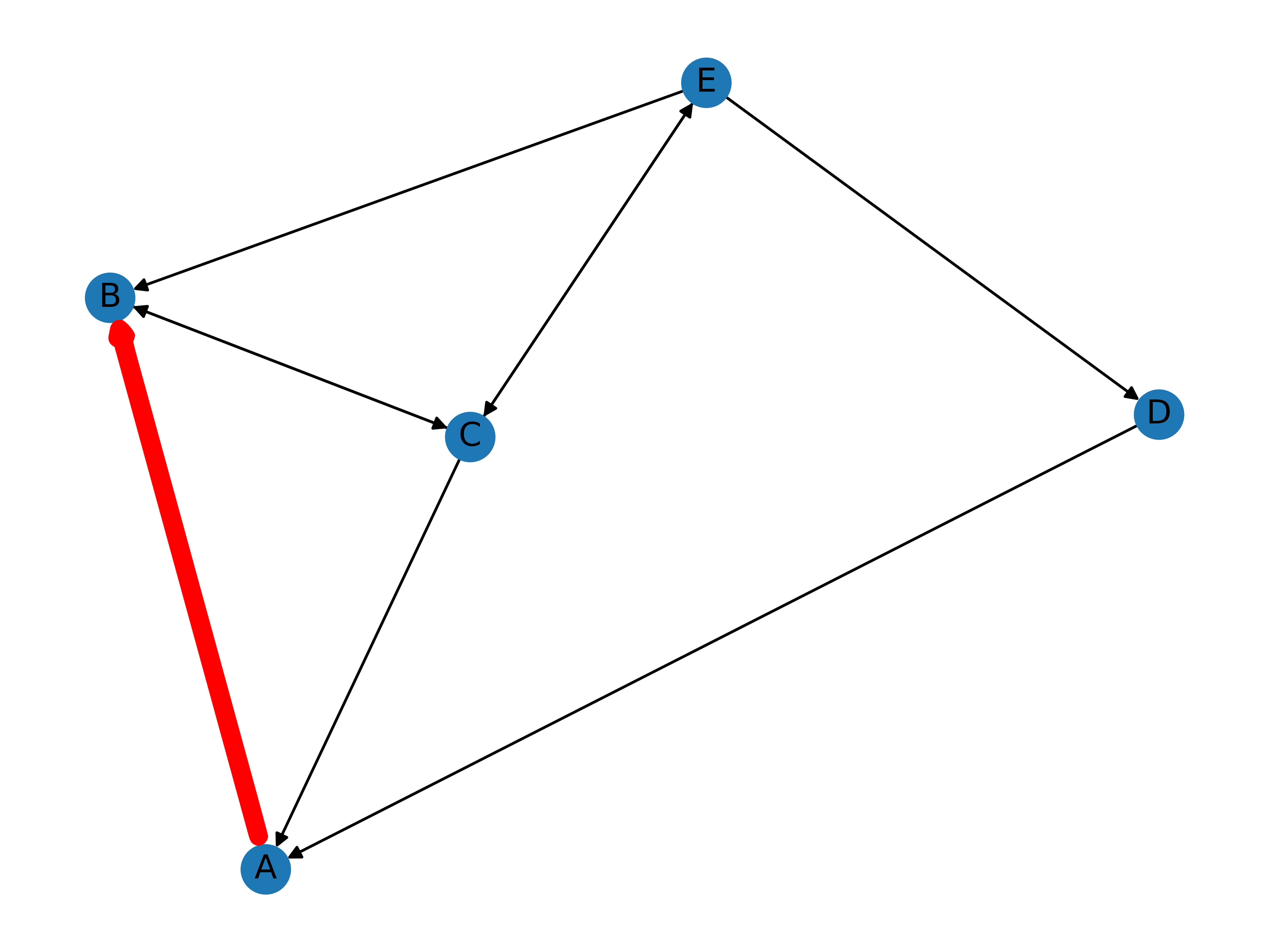
\[Mx_0 = \begin{pmatrix} 0 & 1/2 & 1/3 & 1 & 0 \\ 1 & 0 & 1/3 & 0 & 1/3 \\ 0 & 1/2 & 0 & 0 & 1/3 \\ 0 & 0 & 0 & 0 & 1/3 \\ 0 & 0 & 1/3 & 0 & 0 \end{pmatrix} \cdot \begin{pmatrix} 1 \\ 0 \\ 0 \\ 0 \\ 0 \end{pmatrix} = \begin{pmatrix} 0 \\ 1 \\ 0 \\ 0 \\ 0 \end{pmatrix} = x_1\]

Notice that the result is just the first column of the stochastic matrix, with all entries 0 except for the second one! Why is this the case? Besides the algebraic argument that matrix multiplications can be performed on a column-by-entry basis, the network graph contains the most intuitive answer to our question: there is only one link from page A to page B, which is why \(P(B)\) takes the absolute probability of 1. Simply put, the user clicks on the one and only link on page A to move to page B, as the highlighted path shows.

Once the user reaches page B, however, they now have two choices instead of one: either go back to page A or visit page C. This increase in uncertainty is reflected in the entries of the next vector, \(x_2\):

\[x_2 = Mx_1 = \begin{pmatrix} 0 & 1/2 & 1/3 & 1 & 0 \\ 1 & 0 & 1/3 & 0 & 1/3 \\ 0 & 1/2 & 0 & 0 & 1/3 \\ 0 & 0 & 0 & 0 & 1/3 \\ 0 & 0 & 1/3 & 0 & 0 \end{pmatrix} \cdot \begin{pmatrix} 0 \\ 1 \\ 0 \\ 0 \\ 0 \end{pmatrix} = \begin{pmatrix} 1/2 \\ 0 \\ 1/2 \\ 0 \\ 0 \end{pmatrix}\]

As our intuition suggests, \(P(A) = P(C) = 1/2\), and \(P(A) + P(C) = 1\) since \(A^c = C\). Although no formal proof has been presented, it is now fairly clear that performing this calculation \(n\) times would yield the vector \(x_n\) that contains information about the probability of the user being at websites A, B, C, D, and E, respectively.

Let’s quickly calculate the values of this state vector over some loops.

import numpy as np

def markov_chain(P, x, rep):
	for i in range(rep):
		x = P.dot(x)
	return x

P = np.array([
	[0, 1/2, 1/3, 1, 0], 
	[1, 0, 1/3, 0, 1/3], 
	[0, 1/2, 0, 0, 1/3], 
	[0, 0, 0, 0, 1/3], 
	[0, 0, 1/3, 0, 0]
	])
x_0 = np.array([[1], [0], [0], [0], [0]])
rep = 20

print(markov_chain(P, x_0, rep))

The output of this program is \((0.29270741, 0.39047887, 0.21914571, 0.02430009, 0.07336792)^{T}\). As the Markov process rightly predicts, these numbers each converge to certain values with more repetitions.

\[x_{50} \simeq x_{100} = \begin{pmatrix} 0.29268293 \\ 0.3902439 \\ 0.2195122 \\ 0.02439024 \\ 0.07317073 \end{pmatrix}\]

Also notice that this result is independent of the initial vector we started out with! Suppose a new initial vector x_02 as defined below:

x_02 = np.array([[1/5], [1/5], [1/5], [1/5], [1/5]])

print(markov_chain(P, x_02, rep))

This returns the following output, as expected:

[[0.29268293]
 [0.3902439 ]
 [0.2195122 ]
 [0.02439024]
 [0.07317073]]

There is a mathematical proof behind this fascinating phenomena involving eigenvectors that we will discuss in another post, but there is also an intuitive explanation of this result. Recall that \(x\) was defined as the vector containing the probabilities \(P(A)\), \(P(B)\), \(P(C)\), \(P(D)\), and \(P(E)\). Then, the stationary distribution, \(\lim\limits_{n \to \infty} x_n\), can also be interpreted as the average time that the user spends on a given website. For instance, in our miniature world, the theoretical Internet addict user who sits down on their desk for an infinite number of hours would be expected to spend about \(29\%\) of their time on website A; B, \(39\%\); C, \(22\%\); D, \(2\%\); and E, \(7\%\). Two notable observations might be made about this result. Firstly, the five percentages all add up to a hundred as they should: there are only five websites in the model, and so the probability that the user would be at any one of these five websites is 1. Secondly, \(P(D)\) is the smallest out of the five entries, which aligns with the fact that node D held the most insular position in the network graph. All in all, analyzed from the dimension of time, the notion of stationary distribution is coherent with our intuition that, no matter where the user starts, the average time they spend on each website should be the same given the memoryless nature of the Markov chain.

PageRank Demystified

So we commenced from the seemingly simple question of what PageRank entails. The Markov chain madness may have appeared a bit like a rabbit hole, but it is highly germane to the clockwork behind Google’s search algorithm. Although we used only one parameter—hyperlinks—as the basis of our analysis, in reality PageRank performs batch calculations on a much larger sum of data to ultimately derive the equivalent of our stationary distribution vector. The website that the user is most likely to spend the most time on, i.e. the website that is most likely important and relevant to the user’s search entry, is placed on the top of the list. Other entries follow in sorted order.

So there you have it: the PageRank algorithm demystified. Now the question is, will Google place this post on the top of the search result when a user types “PageRank”? Probably not given the lack of active hyperlinks to and from this webpage. But we’ll see.