Likelihood and Probability

“I think that’s very unlikely.” “No, you’re probably right.”

These are just some of the many remarks we use in every day conversations to express our beliefs. Linguistically, words such as “probably” or “likely” serve to qualify the strength of our professed belief, that is, we express a degree of uncertainty involved with a given statement.

In today’s post, I suggest that we scrutinize the concept of likelihood—what it is, how we calculate it, and most importantly, how different it is from probability. Although the vast majority of us tend to conflate likelihood and probability in daily conversations, mathematically speaking, these two are distinct concepts, though closely related. After concretizing this difference, we then move onto a discussion of maximum likelihood, which is a useful tool frequently employed in Bayesian statistics. Without further ado, let’s jump right in.

Likelihood vs Probability

As we have seen in an earlier post on Bayesian analysis, likelihood tells us—and pardon the circular definition here—how likely a certain parameter is given some data. In other words, the likelihood function answers the question: provided some list of observed or sampled data \(D\), what is the likelihood that our parameter of interest takes on a certain value \(\theta\)? One measurement we can use to answer this question is simply the probability density of the observed value of the random variable at that distribution. In mathematical notation, this idea might be transcribed as:

\[L(\theta \mid D) = P(D \mid \theta) \tag{1}\]

At a glance, likelihood seems to equal probability—after all, that is what the equation (1) seems to suggest. But first, let’s clarify the fact that \(P(D \mid \theta)\) is probability density, not probability. Moreover, the interpretation of probability density in the context of likelihood is different from that which arises when we discuss probability; likelihood attempts to explain the fit of observed data by altering the distribution parameter. Probability, in contrast, primarily deals with the question of how probable the observed data is given some parameter \(\theta\). Likelihood and probability, therefore, seem to ask similar questions, but in fact they approach the same phenomenon from opposite angles, one with a focus on the parameter and the other on data.

Let’s develop more intuition by analyzing the difference between likelihood and probability from a graphical standpoint. To get started, recall the that

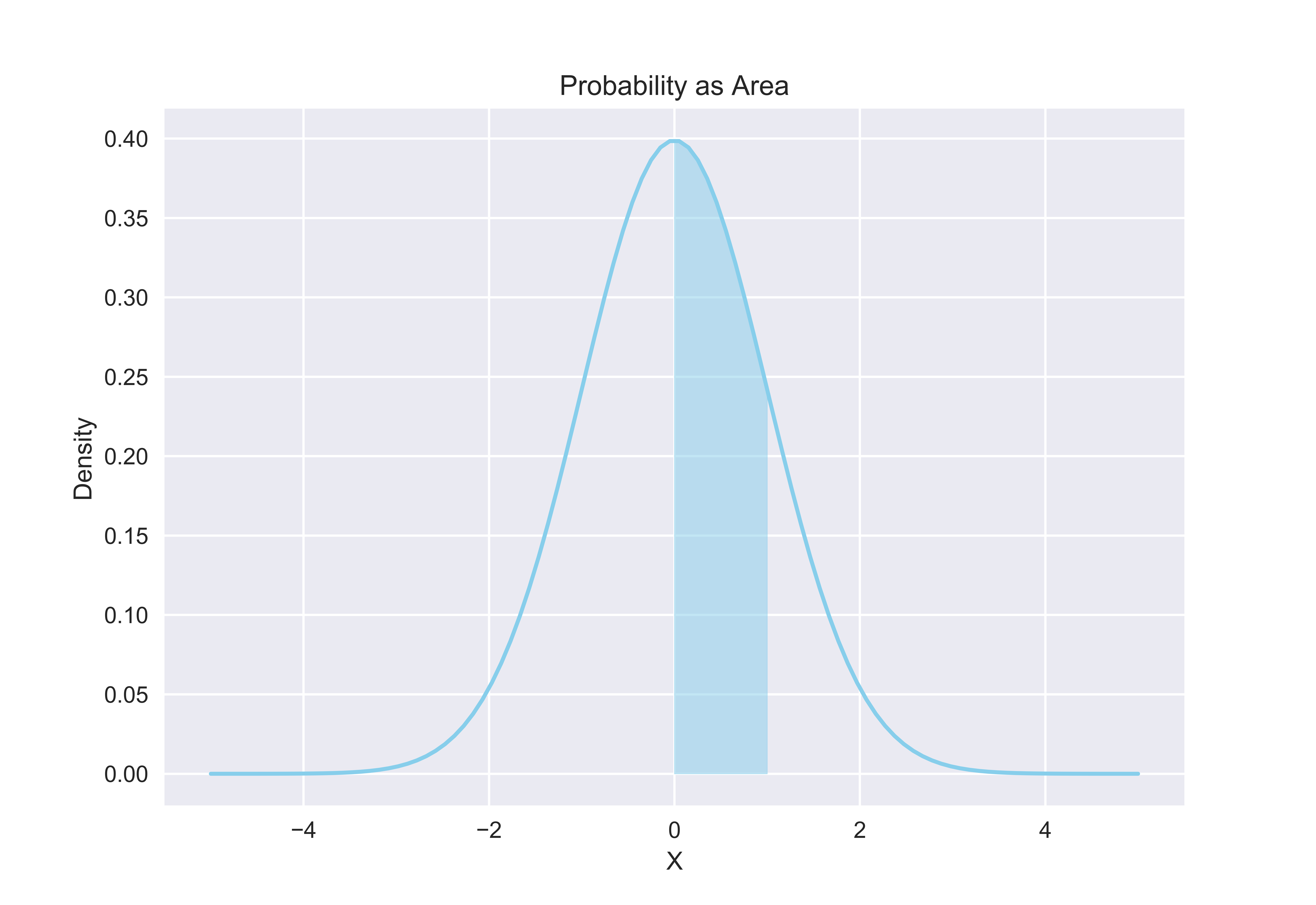
\[P(a < X < b \mid \theta) = \int_a^b f(p) dp\]

This is the good old definition of probability as defined for a continuous random varriable \(X\), given some probability density function \(f(p)\) with parameter \(\theta\). Graphically speaking, we can consider probability as the area or volume under the probability density function, which may be a curve, plane, or a hyperplane depending on the dimensionality of our context.

Figure 1: Representation of probability as area

Unlike probability, likelihood is best understood as a point estimate on the PDF. Imagine having two disparate distributions with distinct parameters. Likelihood is an estimate we can use to see which of these two distributions better explain the data we have in our hands. Intuitively, the closer the mean of the distribution is to the observed data point, the more likely the parameters for the distribution would be. We can see this in action with a simple line of code.

import numpy as np
import matplotlib.pyplot as plt
from scipy.stats import norm

def normal(x, option=True):
    if option:
        mu, sigma = 0, 1
    else:
        mu, sigma = 0.5, 0.7
    return norm.pdf(x, mu,sigma)

x = np.linspace(-5, 5, 100)
p_x = [1, 1]
p_y = [normal(1), normal(1, option=False)]

plt.style.use("seaborn")
plt.plot(x, normal(x), color="skyblue")
plt.plot(x, normal(x, option=False), color="violet")
plt.plot(1, 0, marker='o', color="black")
plt.vlines(p_x, 0, p_y, linestyle="--", color="black", alpha=0.5, linewidth=1.2)
for i, j in zip(p_x, p_y):
    plt.text(i, j, 'L = {:.4f}'.format(j))
plt.title("Likelihood as Height")
plt.xlabel("X")
plt.ylabel("Density")
plt.show()

This code block creates two distributions of different parameters, \(N_1~(1, 0)\) and \(N_2~(0.5, 0.7)\). Then, we assume that a sample of value 1 is observed. Then, we can compare the likelihood of the two parameters given this data by comparing the probability density of the data for each of the two distributions.

Figure 2: Representation of likelihood as height

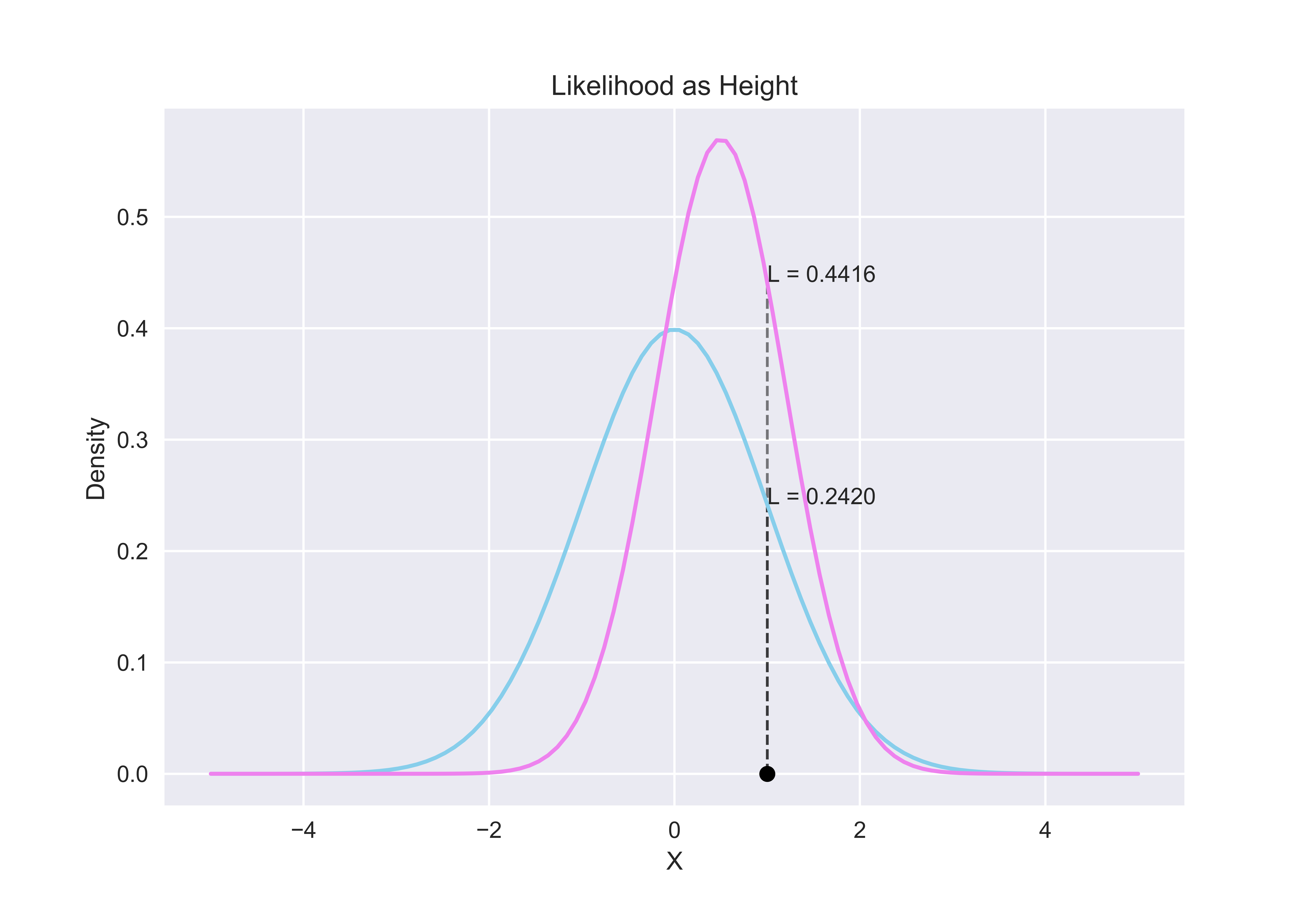
In this case, \(N_2\) seems more likely, i.e. it better explains the data \(X = 1\) since \(L(\theta_{N_1} \mid 1) \approx 0.4416\), which is larger than \(L(\theta_{N_2} \mid 1) \approx 0.2420\).

To sum up, likelihood is something that we can say about a distribution, specifically the parameter of the distribution. On the other hand, probabilities are quantities that we ascribe to individual data. Although these two concepts are easy to conflate, and indeed there exists an important relationship between them explained by Bayes’ theorem, yet they should not be conflated in the world of mathematics. At the end of the day, both of them provide interesting ways to analyze the organic relationship between data and distributions.

Maximum Likelihood

Maximum likelihood estimation, or MLE in short, is an important technique used in many subfields of statistics, most notably Bayesian statistics. As the name suggests, the goal of maximum likelihood estimation is to find the parameters of a distribution that maximizes the probability of observing some given data \(D\). In other words, we want to find the optimal way to fit a distribution to the data. As our intuition suggests, MLE quickly reduces into an optimization problem, the solution of which can be obtained through various means, such as Newton’s method or gradient descent. For the purposes of this post, we look at the simplest way that involves just a bit of calculus.

The best way to demonstrate how MLE works is through examples. In this post, we look at simple examples of maximum likelihood estimation in the context of normal distributions.

Normal Distribution

We have never formally discussed normal distributions on this blog yet, but it is such a widely used, commonly referenced distribution that I decided to jump into MLE with this example. But don’t worry—we will derive the normal distribution in a future post, so if any of this seems overwhelming, you can always come back to this post for reference.

The probability density function for the normal distribution, with parameters \(\mu\) and \(\sigma\), can be written as follows:

\[P(X = x; \mu, \sigma) = \frac{1}{\sqrt{2 \pi \sigma^2}} e^{\frac{-(x - \mu)^2}{2 \sigma^2}}\]

Assume we have a list of observations that correspond to the random variable of interest, \(X\). For each \(x_i\) in the sample data, we can calculate the likelihood of a distribution with parameters \(\theta = (\mu, \sigma)\) by calculating the probability densities at each point of the PDF where \(X = x_i\). We can then make the following statement about these probabilities:

\[L(\theta \mid x_1, x_2, \dots x_n) = P(X = x_1, x_2, \dots x_n \mid \theta) = \prod_{i = 1}^n P(X = x_i \mid \theta)\]

In other words, to maximize the likelihood simply means to find the value of a parameter that which maximizes the product of probabilities of observing each data point. The assumption of independence allows us to use multiplication to calculate the likelihood in this manner. Applied in the context of normal distributions with \(n\) observations, the likelihood function can therefore be calculated as follows:

\[L = \prod_{i = 1}^n \frac{1}{\sqrt{2 \pi \sigma^2}} e^{\frac{-(x_i - \mu)^2}{2 \sigma^2}} \tag{2}\]

But finding the maximum of this function can quickly turn into a nightmare. Recall that we are dealing with distributions here, whose PDFs are not always the simplest and the most elegant-looking. If we multiply \(n\) terms of the normal PDF, for instance, we would end up with a giant exponential term.

Log Likelihood

To prevent this fiasco, we can introduce a simple transformation: logarithms. Log is a monotonically increasing function, which is why maximizing some function \(f\) is equivalent to maximizing the log of that function, \(\log(f)\). Moreover, the log transformation expedites calculation since logarithms restructure multiplication as sums.

\[\log ab = \log a + \log b \tag{3}\]

With that in mind, we can construct a log equation for MLE from (3) as shown below. Because we are dealing with Euler’s number, \(e\), the natural log is our preferred base.

\[\ln L = \ln \frac{1}{(2 \pi \sigma)^n} e^{\frac{\sum_{i = 1}^n (x_i - \mu)^2}{2 \sigma^2}}\]

Using the property in (3), we can simplify the equation above:

\[\ln L = \ln \frac{1}{(2 \pi \sigma)^n} + \ln e^{\frac{\sum_{i = 1}^n (x_i - \mu)^2}{2 \sigma^2}} = - \frac{n}{2} \ln 2 \pi - n \ln \sigma - \frac{1}{2 \sigma^2} \sum_{i = 1}^n (x_i - \mu)^2 \tag{4}\]

Maximum Likelihood Estimation

To find the maximum of this function, we can use a bit of calculus. Specifically, our goal is to find a parameter that which makes the first derivative of the log likelihood function to equal 0. To find the optimal mean parameter \(\mu\), we derive the log likelihood function with respect to \(\mu\) while considering all other variables as constants.

\[\frac{d}{d \mu} \ln L = 0 + 0 + \frac{\sum_{i = 1}^n 2(x_i - \mu)}{2 \sigma^2} = \frac{\sum_{i = 1}^n x_i - \mu}{\sigma^2} = 0\]

From this, it follows that

\[\frac{1}{\sigma^2}[(x_1 + x_2 + \dots + x_n) - n \mu] = 0\]

Rearranging this equation, we are able to obtain the final expression for the optimal parameter \(\mu\) that which maximizes the likelihood function:

\[\mu = \frac{\sum_{i = 1}^n x_i}{n} \tag{5}\]

As part 2 of the trilogy, we can also do the same for the other parameter of interest in the normal distribution, namely the standard deviation denoted by \(\sigma\).

\[\frac{d}{d \sigma} \ln L = - \frac{n}{\sigma} + \frac{\sum_{i = 1}^n (x_i - \mu)^2}{\sigma^3} = 0\]

We can simplify this equation by multiplying both sides by \(\sigma^3\). After a little bit of rearranging, we end up with

\[\sigma = \sqrt \frac{\sum_{i = 1}^n (x_i - \mu)^2}{n} \tag{6}\]

Finally, we have obtained the parameter values for the mean and variance of a normal distribution that maximizes the likelihood of our data. Notice that, in the context of normal distributions, the ML parameters are simply the mean and standard deviation of the given data point, which closely aligns with our intuition: the normal distribution that best explains given data would have the sample mean and variance as its parameters, which is exactly what our result suggests. Beyond the specific context of normal distributions, however, MLE is generally very useful when trying to reconstruct or approximate the population distribution using observed data.

In Code

Let’s wrap this up by performing a quick verification of our formula for maximum likelihood estimation for normal distributions. First, we need to prepare some random numbers that will serve as our supposed observed data.

import numpy as np
import matplotlib.pyplot as plt

np.random.seed(123)
num_list = np.random.randint(low=0, high=10, size=10).tolist()

We then calculate the optimum parameters \(\mu\) and \(\sigma\) by using the formulas we have derived in (5) and (6).

mu_best = np.mean(num_list)
sigma_best = np.std(num_list)

We then generate two subplots of the log likelihood function as expressed in (4), where we vary \(\mu\) while keeping \(\sigma\) at sigma_best in one and flip this in the other. This can be achieved in the following manner.

n = len(num_list)
x_mu = np.linspace(1, 10, 10)
x_sigma = np.linspace(1, 10, 10)
y_mu = [-n/2 * np.log(2 * np.pi) - n * np.log(sigma_best) - 1/(2 * sigma_best**2) * np.sum((num_list - i)**2) for i in x_mu]
y_sigma = -n/2 * np.log(2 * np.pi)- n * np.log(x_sigma) - 1/(2 * x_sigma**2) * np.sum((num_list - mu_best)**2)

plt.style.use("seaborn")
fig, ax = plt.subplots(nrows=1, ncols=2, figsize=(5, 3))
ax[0].plot(x_mu, y_mu, color="skyblue")
ax[0].set(xlabel="$\\mu$",ylabel="Log Likelihood")
ax[0].axvline(mu_best, 0, 1, color="black", ls="--", lw=1)
ax[1].plot(x_sigma, y_sigma, color="skyblue")
ax[1].set(xlabel="$\\sigma$",ylabel="")
ax[1].axvline(sigma_best, 0, 1, color="black", ls="--", lw=1)

plt.tight_layout()
plt.show()

Executing this code block produces the figure below.

Figure: Log likelihood for mean and standard deviation

From the graph, we can see that the maximum occurs at the mean and standard deviation of the distribution as we expect. Combining these two results, we would expect the maximum likelihood distribution to follow \(N~(\mu, \sigma)\) where \(\mu\) = mu_best and \(\sigma\) = sigma_best in our code.

Conclusion

And that concludes today’s article on (maximum) likelihood. This post was motivated from a rather simple thought that came to my mind while overhearing a conversation that happened at the PMO office. Despite the conceptual difference between probability and likelihood, people will continue to use employ these terms interchangeably in daily conversations. From a mathematician’s point of view, this might be unwelcome, but the vernacular rarely strictly aligns with academic lingua. In fact, it’s most often the reverse; when jargon or scholarly terms get diffused with everyday language, they often transform in meaning and usage. I presume words such as “likelihood” or “likely” fall into this criteria. All of this notwithstanding, I hope this post provided you with a better understanding of what likelihood is, and how it relates to other useful statistical concepts such as maximum likelihood estimation.

The topic for our next post is going to be Monte Carlo simulations and methods. If “Monte Carlo” just sounds cool to you, as it did to me when I first came across it, tune in again next week. Catch you up in the next one.