So What are Autoencoders?
In today’s post, we will take yet another look at an interesting application of a neural network: autoencoders. There are many types of autoencoders, but the one we will be looking at today is the simplest variant, the vanilla autoencoder. Despite its simplicity, however, there is a lot of insight to glean from this example—in fact, it is precisely the simplicity that allows us to better understand how autoencoders work, and potentially extend that understanding to to analyze other flavors of autoencoders, such as variational autoencoder networks which we might see in a future post. Without further ado, let’s get started.
Building the Model
We begin by importing all modules and configurations necessary for this tutorial.
import os
import datetime
import numpy as np
from tensorflow.keras import datasets
from tensorflow.keras.layers import *
from tensorflow.keras.models import Model
from tensorflow.keras.utils import plot_model
from tensorflow.keras import callbacks
%load_ext tensorboard
%matplotlib inline
%config InlineBackend.figure_format = 'svg'
import matplotlib.pyplot as plt
plt.style.use('seaborn')
Latent Dimension
How do autoencoders work? There are entire books dedicated to this topic, and this post in no way claims to introduce and explore all the fascinating complexities of this model. However, one intuitive way to understand autoencoders is to consider them as, lo and behold, encoders that map complex data points into vectors living in some latent dimension.
For example, a 28-by-28 pixel RGB channel image might be compressed into a five-dimensional latent vector. The five numbers composing this vector somehow encodes the core information needed to then decode this vector back into the original 28-by-28 pixel RGB channel image. Of course, some information is inevitably going to be lost—after all, how can five numbers describe the entirety of an image? However, what’s important and fascinating about autoencoders is that, with appropriate training and configuration, they manage to find ways to best compress input data into latent vectors that can be decoded to regenerate a close approximation of the input data.
For the purposes of this demonstration, let’s configure the latent dimension of the encoder to be 128 dimensions—in other words, each 28-by-28, single-channel image will be encoded into vectors living in 128 dimensional space.
compressed_dim = 128
image_shape = (28, 28, 1)
Encoder-Decoder Model
It’s time to build the autoencoder model. In summary, an autoencoder is composed of two components: an encoder and a decoder. The encoder transfers input data into the latent dimension, and the decoder performs the exact reverse: it takes vectors in the latent space and rearranges it to bring it back into its original dimension, which is, in this case, a 28-by-28, single-channel image.
The followign code snippet implements this logic using the tf.keras functional API.
def build_model(image_shape, compressed_dim):
  encoder_input = Input(shape=image_shape)
  x = Conv2D(16, 3, activation='relu', padding='same')(encoder_input)
  x = BatchNormalization()(x)
  x = MaxPooling2D(2, padding='same')(x)
  x = Conv2D(32, 3, activation='relu', padding='same')(x)
  x = BatchNormalization()(x)
  x = MaxPooling2D(2, padding='same')(x)
  x = Conv2D(32, 3, activation='relu', padding='same')(x)
  x = Flatten()(x)
  encoder_output = Dense(compressed_dim, activation='sigmoid')(x)
  x = Dense(7 * 7 * 32, activation='relu')(encoder_output)
  x = Reshape((7, 7, 32))(x)
  x = Conv2DTranspose(32, 3, activation='relu', padding='same')(x)
  x = BatchNormalization()(x)
  x = UpSampling2D(2)(x)
  x = Conv2DTranspose(32, 3, activation='relu', padding='same')(x)
  x = BatchNormalization()(x)
  x = UpSampling2D(2)(x)
  x = Conv2DTranspose(16, 3, activation='relu', padding='same')(x)
  decoder_output = Conv2D(1, 3, activation='sigmoid', padding='same')(x)
  encoder = Model(encoder_input, encoder_output)
  autoencoder = Model(encoder_input, decoder_output)
  autoencoder.compile(optimizer='adam', loss='binary_crossentropy')
  print(autoencoder.summary())
  return encoder, autoencoder
Let’s declare the encoder and autoencoder model by invoking the build_model function with the specified image shape and the dimensionality of the latent space.
encoder, autoencoder = build_model(image_shape, compressed_dim)
Just to get a sense of what operations are taking place dimensionality-wise, here is a look at the output shapes of the autoencoder model. Notice that the input is of shape (None, 28, 28, 1), and that the final output is also of the same shape (None, 28, 28, 1), as expected.
Model: "model"
_________________________________________________________________
Layer (type)                 Output Shape              Param #
=================================================================
input_1 (InputLayer)         [(None, 28, 28, 1)]       0
_________________________________________________________________
conv2d (Conv2D)              (None, 28, 28, 16)        160
_________________________________________________________________
batch_normalization (BatchNo (None, 28, 28, 16)        64
_________________________________________________________________
max_pooling2d (MaxPooling2D) (None, 14, 14, 16)        0
_________________________________________________________________
conv2d_1 (Conv2D)            (None, 14, 14, 32)        4640
_________________________________________________________________
batch_normalization_1 (Batch (None, 14, 14, 32)        128
_________________________________________________________________
max_pooling2d_1 (MaxPooling2 (None, 7, 7, 32)          0
_________________________________________________________________
conv2d_2 (Conv2D)            (None, 7, 7, 32)          9248
_________________________________________________________________
flatten (Flatten)            (None, 1568)              0
_________________________________________________________________
dense (Dense)                (None, 128)               200832
_________________________________________________________________
dense_1 (Dense)              (None, 1568)              202272
_________________________________________________________________
reshape (Reshape)            (None, 7, 7, 32)          0
_________________________________________________________________
conv2d_transpose (Conv2DTran (None, 7, 7, 32)          9248
_________________________________________________________________
batch_normalization_2 (Batch (None, 7, 7, 32)          128
_________________________________________________________________
up_sampling2d (UpSampling2D) (None, 14, 14, 32)        0
_________________________________________________________________
conv2d_transpose_1 (Conv2DTr (None, 14, 14, 32)        9248
_________________________________________________________________
batch_normalization_3 (Batch (None, 14, 14, 32)        128
_________________________________________________________________
up_sampling2d_1 (UpSampling2 (None, 28, 28, 32)        0
_________________________________________________________________
conv2d_transpose_2 (Conv2DTr (None, 28, 28, 16)        4624
_________________________________________________________________
conv2d_3 (Conv2D)            (None, 28, 28, 1)         145
=================================================================
Total params: 440,865
Trainable params: 440,641
Non-trainable params: 224
_________________________________________________________________
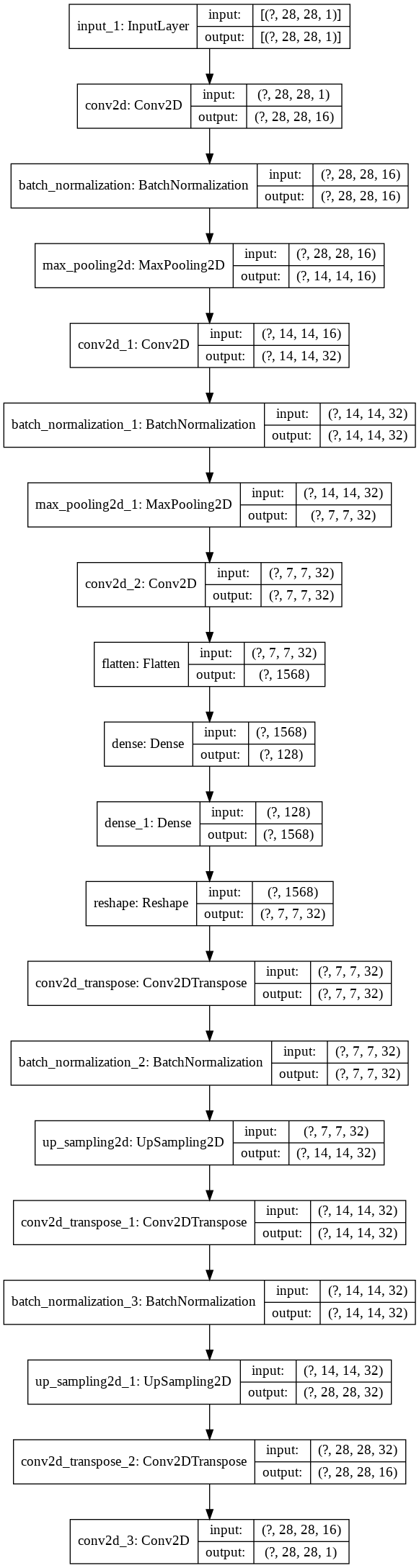
Here’s the image of the model for the fancy bells and whistles.
plot_model(autoencoder, show_shapes=True, show_layer_names=True)
Now that the autoencoder model is fully ready, it’s time to see what it can do!
Testing the Autoencoder
Although autoencoders present countless exciting possibilities for application, we will look at a relatively simple use of an autoencoder in this post: denoising. There might be times when the photos we take or image data we use are tarnished by noise—undesired dots or lines that undermine image quality. An autoencoder can be trained to remove these noises fairly easily as we will see in thi post.
Data Preparation
First, let’s import the MNIST data set for this tutorial. Nothing much exciting is happening below, except for the fact that we are rearranging and preprocessing the dataset so as to maximize training efficiency.
def load_data():
  (X_train, _), (X_test, _) = datasets.mnist.load_data()
  X_train = np.reshape(X_train, (len(X_train), 28, 28, 1))
  X_test = np.reshape(X_test, (len(X_test), 28, 28, 1))
  X_train, X_test = X_train.astype('float64') / 255., X_test.astype('float64') / 255.
  return X_train, X_test
X_train, X_test = load_data()
Next, we will add noise to the data. Note that the MNIST dataset does not contain noise by default: we will have to artificially and intentionally tarnish the dataset to produce a noisy training set for the autoencoder model. The add_noise function precisely performs this function.
def add_noise(data, noise_factor):
  data_noise = data + noise_factor * np.random.normal(size=data.shape)
  data_noise = np.clip(data_noise, 0., 1.)
  return data_noise
Using the add_noise function, we can create a noisy sample. Note that noise_factor was set to 0.5, although I’d imagine other values within reasonable range would work equally well as well.
X_train_noise = add_noise(X_train, 0.5)
Model Training
Training the model is very simple: the training data is X_train_noise, the noisy dataset, and the predicted label is X_train. Through this configuration, we essentially expect the autoencoder to be able to see noisy images, after which encoding and decoding is performed via a transformation to a latent dimension to ultimately reproduce a pristine image devoid of any noise.
For experimental puposes, I tried using the TensorBoard callback on Google Colab. TensorBoard is a platform that gives developers full view of what happens during and after the training process. It makes observing metrics like loss and accuracy a breeze. I highly recommend that you check out this tutorial on how to use and configure this functionality on your notebook.
log_dir = os.path.join("logs", datetime.datetime.now().strftime("%Y%m%d-%H%M%S"))
callback = callbacks.TensorBoard(log_dir, histogram_freq=0)

history = autoencoder.fit(X_train_noise, X_train,
                          epochs=35,
                          batch_size=64,
                          shuffle=True,
                          validation_split=0.1,
                          callbacks=[callback])
Train on 54000 samples, validate on 6000 samples
Epoch 1/35
54000/54000 [==============================] - 9s 170us/sample - loss: 0.1358 - val_loss: 0.1091
Epoch 2/35
54000/54000 [==============================] - 6s 117us/sample - loss: 0.1046 - val_loss: 0.1041
Epoch 3/35
54000/54000 [==============================] - 6s 118us/sample - loss: 0.1004 - val_loss: 0.1001
Epoch 4/35
54000/54000 [==============================] - 6s 118us/sample - loss: 0.0982 - val_loss: 0.1001
Epoch 5/35
54000/54000 [==============================] - 6s 116us/sample - loss: 0.0966 - val_loss: 0.0995
Epoch 6/35
54000/54000 [==============================] - 6s 117us/sample - loss: 0.0956 - val_loss: 0.0991
Epoch 7/35
54000/54000 [==============================] - 6s 117us/sample - loss: 0.0946 - val_loss: 0.0969
Epoch 8/35
54000/54000 [==============================] - 6s 117us/sample - loss: 0.0939 - val_loss: 0.0971
Epoch 9/35
54000/54000 [==============================] - 6s 117us/sample - loss: 0.0932 - val_loss: 0.0966
Epoch 10/35
54000/54000 [==============================] - 6s 117us/sample - loss: 0.0928 - val_loss: 0.0959
Epoch 11/35
54000/54000 [==============================] - 6s 116us/sample - loss: 0.0922 - val_loss: 0.0966
Epoch 12/35
54000/54000 [==============================] - 6s 117us/sample - loss: 0.0917 - val_loss: 0.0958
Epoch 13/35
54000/54000 [==============================] - 6s 116us/sample - loss: 0.0914 - val_loss: 0.0958
Epoch 14/35
54000/54000 [==============================] - 6s 116us/sample - loss: 0.0910 - val_loss: 0.0970
Epoch 15/35
54000/54000 [==============================] - 6s 116us/sample - loss: 0.0907 - val_loss: 0.0961
Epoch 16/35
54000/54000 [==============================] - 6s 116us/sample - loss: 0.0903 - val_loss: 0.0983
Epoch 17/35
54000/54000 [==============================] - 6s 118us/sample - loss: 0.0900 - val_loss: 0.0987
Epoch 18/35
54000/54000 [==============================] - 7s 121us/sample - loss: 0.0898 - val_loss: 0.0963
Epoch 19/35
54000/54000 [==============================] - 6s 116us/sample - loss: 0.0895 - val_loss: 0.0953
Epoch 20/35
54000/54000 [==============================] - 6s 116us/sample - loss: 0.0893 - val_loss: 0.0959
Epoch 21/35
54000/54000 [==============================] - 6s 117us/sample - loss: 0.0890 - val_loss: 0.0954
Epoch 22/35
54000/54000 [==============================] - 6s 116us/sample - loss: 0.0888 - val_loss: 0.0953
Epoch 23/35
54000/54000 [==============================] - 6s 116us/sample - loss: 0.0887 - val_loss: 0.0954
Epoch 24/35
54000/54000 [==============================] - 6s 117us/sample - loss: 0.0885 - val_loss: 0.0958
Epoch 25/35
54000/54000 [==============================] - 6s 117us/sample - loss: 0.0882 - val_loss: 0.0958
Epoch 26/35
54000/54000 [==============================] - 6s 116us/sample - loss: 0.0880 - val_loss: 0.0966
Epoch 27/35
54000/54000 [==============================] - 6s 117us/sample - loss: 0.0879 - val_loss: 0.0956
Epoch 28/35
54000/54000 [==============================] - 6s 116us/sample - loss: 0.0877 - val_loss: 0.0956
Epoch 29/35
54000/54000 [==============================] - 6s 116us/sample - loss: 0.0876 - val_loss: 0.0954
Epoch 30/35
54000/54000 [==============================] - 6s 117us/sample - loss: 0.0874 - val_loss: 0.0959
Epoch 31/35
54000/54000 [==============================] - 6s 118us/sample - loss: 0.0873 - val_loss: 0.0959
Epoch 32/35
54000/54000 [==============================] - 6s 116us/sample - loss: 0.0872 - val_loss: 0.0960
Epoch 33/35
54000/54000 [==============================] - 6s 116us/sample - loss: 0.0871 - val_loss: 0.0958
Epoch 34/35
54000/54000 [==============================] - 6s 117us/sample - loss: 0.0869 - val_loss: 0.0980
Epoch 35/35
54000/54000 [==============================] - 6s 116us/sample - loss: 0.0867 - val_loss: 0.0981
The Result
Now that the training is over, what can we do with this autoencoder? Well, let’s see if the autoencoder is now capable of removing noise from tainted image files. But before we jump right into that, let’s first build a simple function that displays images for our convenience.
def show_image(data, num_row):
  num_image = num_row**2
  plt.figure(figsize=(10,10))
  for i in range(num_image):
    plt.subplot(num_row,num_row,i+1)
    plt.grid(False)
    plt.xticks([]); plt.yticks([])
    data_point = data[i].reshape(28, 28)
    plt.imshow(data_point, cmap=plt.cm.binary)
  plt.show()
Using the show_image function, we can now display 25 test images that we will feed into the autoencoder.
show_image(X_test, 5)

Let’s add noise to the data.
X_test_noise = add_noise(X_test, 0.5)
show_image(X_test_noise, 5)

Finally, the time has come! The autoencoder will try to “denoise” the contaminated images. Let’s see if it does a good job.
denoised_images = autoencoder.predict(X_test_noise)
show_image(denoised_images, 5)

Lo and behold, the autoencoder produces pristine images, almost reverting them back to their original state!
Conclusion
I find autoencoders interesting for two reasons. First, they can be used to compress images into lower dimensions. Our original image was of size 28-by-28, summing up to a total of 784 pixels. Somehow, the autoencoder finds ways to decompress this image into vectors living in the predefined 128 dimensions. This is interesting in and of itself, since it presents ways that we might be able to compress large files with minimal loss of information. But more importantly, as we have seen in this tutorial, autoencoders can be used to perform certain tasks, such as removing noise from data, and many more.
In the next post, we will take a look at a variant of this vanilla autoencoder model, known as variational autoencoders. Variataional autoencoders are a lot more powerful and fascinating because they can actually be used to generate data instead of merely processing them.
I hope you enjoyed reading this post. Stay tuned for more!