A Simple Autocomplete Model

You might remember back in the old days when autocomplete was just terrible. The suggestions provided by autocomplete would be useless if not downright stupid—I remember that one day when I intended to type “Gimme a sec,” only to see my message get edited into “Gimme a sex” by the divine touches of autocomplete. On the same day, the feature was turned off on my phone for the betterment of the world.

Now, times have changed. Recently, I decided to give autocorrect a chance on my iPhone. Surprisingly, I find myself liking autocomplete more than hating it, especially now that the weather is getting colder by each day: when my frost-numbed finger tips touch on the wrong places of the phone screen to produce words that aren’t really words, iPhone’s autocomplete somehow magically reads my mind to rearrange all that inscrutable alphabet soup into words that make actual, coherent sense. Sometimes, it’s so good at correcting my typos that I intentionnally make careless mistakes on the keyboard just to see how far it can go.

One of the obvious reasons behind such drastic improvements in autocomplete functionality is the development of deep neural networks. As we know, neural networks are great at learning hidden patterns as long as we feed it with enough data. In this post, we will implement a very simple version of a generative deep neural network that can easily form the backbone of some character-based autocomplete algorithm. Let’s begin!

Data Preparation

Let’s first go ahead and import all dependencies for this tutorial. As always, we will be using the tensorflow.keras functional API to build our neural network.

import numpy as np
import tensorflow as tf
from tensorflow.keras import layers
from tensorflow.keras.models import Model, load_model
from tensorflow.keras.utils import plot_model
%matplotlib inline
%config InlineBackend.figure_format = 'svg'
import matplotlib.pyplot as plt
plt.style.use('seaborn')

Loading Data

We will be training our neural network to speak like the great German philosopher Friedrich Nietzsche (or his English translations, to be more exact). First, let’s build a function that retrieves the necessary .txt text file document from the web to return a Python string.

def get_text():
  path = tf.keras.utils.get_file('nietzsche.txt',
                               origin='https://s3.amazonaws.com/text-datasets/nietzsche.txt') 
  text = open(path).read().lower()
  return text

Let’s take a look at the text data by examining its length.

text_data = get_text()
print("Character length: {0}".format(len(text_data)))

Character length: 600893

Just to make sure that the data has been loaded successfully, let’s take a look at the first 100 characters of the string.

print(text_data[:100])

preface

 supposing that truth is a woman--what then? is there not ground 
 for suspecting that all ph

## Preprocessing

It’s time to preprocess the text data to make it feedable to our neural network. As introduced in this previous post on recurrent neural networks, the smart way to deal with text preprocessing is typically to use an embedding layer that translates words into vectors. However, text embedding is insuitable for this task since our goal is to build a character-level text generation model. In other words, our model is not going to generate word predictions; instead, it will spit out a character each prediction cycle. Therefore, we will use an alternative technique, namely mapping each character to an integer value. This isn’t as elegant as text embedding or even one-hot encoding but for a character-level analysis, it should work fine. The preprocess_split function takes a string text data as input and returns a list of training data, each of length max_len, sampled every step characters. It also returns the training labels and a hash table mapping characters to their respective integer encodings.

def preprocess_split(text, max_len, step):
  sentences, next_char = [], []
  for i in range(0, len(text) - max_len, step):
    sentences.append(text[i: i + max_len])
    next_char.append(text[i + max_len])
  char_lst = sorted(list(set(text)))
  char_dict = {char: char_lst.index(char) for char in char_lst}
  X = np.zeros((len(sentences), max_len, len(char_lst)), dtype=np.bool)
  y = np.zeros((len(next_char), len(char_lst)), dtype=np.bool)
  for i, sentence in enumerate(sentences):
    for j, char in enumerate(sentence):
      X[i, j, char_dict[char]] = 1
    y[i, char_dict[next_char[i]]] = 1
  return X, y, char_dict

Let’s perform a quick sanity check to see if the function works as expected. Specifying max_len to 60 means that each instance in the training data will be 60 consecutive characters sampled from the text data every step characters.

max_len = 60
step = 3
X, y, char_dict = preprocess_split(text_data, max_len, step)
vocab_size = len(char_dict)
print("Number of sequences: {0}\nNumber of unique characters: {1}".format(len(X), vocab_size))

Number of sequences: 200278
Number of unique characters: 57

The result tells us that we have a total of 200278 training instances, which is probably plenty to train, test, and validate our model. The result also tells us that there are 57 unique characters in the text data. Note that these unique characters not only include alphabets but also r'\tab'and other miscellaneous white spacing characters and punctuations.

Model Training

Model Design

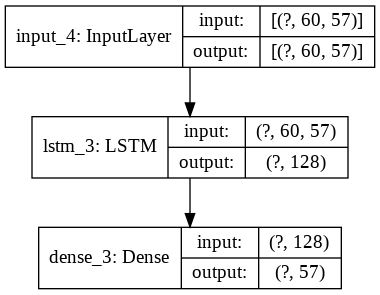
Let’s now design our model. Because there is obviously going to be sequential, temporal structure underlying the training data, we will use an LSTM layer, a type of advanced recurrent neural network we saw in the previous post. In fact, this is all we need, unless we want to create a deep neural network spanning multiple layers. However, training such a model would cost a lot of time and computational resource. For the sake of simplicity, we will build a simple model with a single LSTM layer. The output layer is going to be a dense layer with vocab_size number of neurons, activated with a softmax function. We can thus interpret the index of the biggest value of the final array to correspond to the most likely character.

def build_model(max_len, vocab_size):
  inputs = layers.Input(shape=(max_len, vocab_size))
  x = layers.LSTM(128)(inputs)
  output = layers.Dense(vocab_size, activation=tf.nn.softmax)(x)
  model = Model(inputs, output)
  model.compile(optimizer='adam', loss='categorical_crossentropy')
  return model

model = build_model(max_len, vocab_size)
plot_model(model, show_shapes=True, show_layer_names=True)

Below is a full plot of the model that shows the dimensions of the input and output tensors of all layers.

Model Training

Now, all we have to do is to train the model with the data. Let’s run this for 50 epochs, just to give our model enough time to explore the loss function and settle on a good minimum.

history = model.fit(X, y, epochs=50, batch_size=128)

Train on 200278 samples
Epoch 1/50
200278/200278 [==============================] - 164s 817us/sample - loss: 2.5568
Epoch 2/50
200278/200278 [==============================] - 163s 813us/sample - loss: 2.1656
Epoch 3/50
200278/200278 [==============================] - 162s 810us/sample - loss: 2.0227
Epoch 4/50
200278/200278 [==============================] - 162s 809us/sample - loss: 1.9278
Epoch 5/50
200278/200278 [==============================] - 161s 805us/sample - loss: 1.8586
Epoch 6/50
200278/200278 [==============================] - 162s 811us/sample - loss: 1.8032
Epoch 7/50
200278/200278 [==============================] - 163s 815us/sample - loss: 1.7582
Epoch 8/50
200278/200278 [==============================] - 165s 825us/sample - loss: 1.7197
Epoch 9/50
200278/200278 [==============================] - 167s 833us/sample - loss: 1.6866
Epoch 10/50
200278/200278 [==============================] - 166s 830us/sample - loss: 1.6577
Epoch 11/50
200278/200278 [==============================] - 165s 823us/sample - loss: 1.6312
Epoch 12/50
200278/200278 [==============================] - 162s 810us/sample - loss: 1.6074
Epoch 13/50
200278/200278 [==============================] - 162s 811us/sample - loss: 1.5862
Epoch 14/50
200278/200278 [==============================] - 161s 805us/sample - loss: 1.5668
Epoch 15/50
200278/200278 [==============================] - 165s 822us/sample - loss: 1.5492
Epoch 16/50
200278/200278 [==============================] - 166s 829us/sample - loss: 1.5333
Epoch 17/50
200278/200278 [==============================] - 167s 832us/sample - loss: 1.5182
Epoch 18/50
200278/200278 [==============================] - 166s 828us/sample - loss: 1.5051
Epoch 19/50
200278/200278 [==============================] - 166s 827us/sample - loss: 1.4922
Epoch 20/50
200278/200278 [==============================] - 164s 819us/sample - loss: 1.4801
Epoch 21/50
200278/200278 [==============================] - 165s 826us/sample - loss: 1.4688
Epoch 22/50
200278/200278 [==============================] - 165s 826us/sample - loss: 1.4582
Epoch 23/50
200278/200278 [==============================] - 165s 822us/sample - loss: 1.4488
Epoch 24/50
200278/200278 [==============================] - 163s 813us/sample - loss: 1.4386
Epoch 25/50
200278/200278 [==============================] - 167s 832us/sample - loss: 1.4305
Epoch 26/50
200278/200278 [==============================] - 166s 830us/sample - loss: 1.4220
Epoch 27/50
200278/200278 [==============================] - 167s 832us/sample - loss: 1.4137
Epoch 28/50
200278/200278 [==============================] - 167s 833us/sample - loss: 1.4060
Epoch 29/50
200278/200278 [==============================] - 166s 827us/sample - loss: 1.3989
Epoch 30/50
200278/200278 [==============================] - 164s 820us/sample - loss: 1.3910
Epoch 31/50
200278/200278 [==============================] - 163s 815us/sample - loss: 1.3846
Epoch 32/50
200278/200278 [==============================] - 162s 810us/sample - loss: 1.3777
Epoch 33/50
200278/200278 [==============================] - 162s 809us/sample - loss: 1.3720
Epoch 34/50
200278/200278 [==============================] - 160s 798us/sample - loss: 1.3649
Epoch 35/50
200278/200278 [==============================] - 163s 815us/sample - loss: 1.3599
Epoch 36/50
200278/200278 [==============================] - 162s 807us/sample - loss: 1.3538
Epoch 37/50
200278/200278 [==============================] - 162s 808us/sample - loss: 1.3482
Epoch 38/50
200278/200278 [==============================] - 162s 809us/sample - loss: 1.3423
Epoch 39/50
200278/200278 [==============================] - 163s 813us/sample - loss: 1.3371
Epoch 40/50
200278/200278 [==============================] - 164s 820us/sample - loss: 1.3319
Epoch 41/50
200278/200278 [==============================] - 163s 814us/sample - loss: 1.3268
Epoch 42/50
200278/200278 [==============================] - 165s 825us/sample - loss: 1.3223
Epoch 43/50
200278/200278 [==============================] - 164s 820us/sample - loss: 1.3171
Epoch 44/50
200278/200278 [==============================] - 164s 819us/sample - loss: 1.3127
Epoch 45/50
200278/200278 [==============================] - 165s 822us/sample - loss: 1.3080
Epoch 46/50
200278/200278 [==============================] - 163s 813us/sample - loss: 1.3034
Epoch 47/50
200278/200278 [==============================] - 163s 813us/sample - loss: 1.2987
Epoch 48/50
200278/200278 [==============================] - 162s 809us/sample - loss: 1.2955
Epoch 49/50
200278/200278 [==============================] - 161s 804us/sample - loss: 1.2905
Epoch 50/50
200278/200278 [==============================] - 162s 811us/sample - loss: 1.2865

Saving the Model

As I was training this model on Google Colab, I noticed that training even this simple model took a lot of time. Therefore, I decided that it is a good idea to probably save the trained model—in the worst case scenario that poor network connection suddenly caused the Jupyter kernel to die, saving a saved model file would be of huge help since I can continue training again from there.

Saving the model on Google Colab requires us to import a simple module, google.colab. The process is very simple.

from google.colab import files

model = model.save('model.hdf5')
files.download('model.hdf5')

To load the model, we can simply call the command below.

model = load_model('model.hdf5')

Learning Curve

Let’s take a look at the loss curve of the model. We can simply look at the value of the loss function as printed throughout the training scheme, but why not visualize it if we can?

def plot_learning_curve(history):
  loss = history.history['loss']
  epochs = [i for i, _ in enumerate(loss)]
  plt.scatter(epochs, loss, color='skyblue')
  plt.xlabel('Epochs'); plt.ylabel('Cross Entropy Loss')
  plt.show()

plot_learning_curve(history)

As expected, the loss decreases throughout each epoch. The reason I was not paticularly worried about overfitting was that we had so much data to work with, especially in comparison with the relatively constrained memory capacity of our one-layered model.

Prediction Generation

One of the objectives of this tutorial was to demonstrate the fun we can have with generative models, namely neural networks that can be used to generate data themselves, not just classify or predict data points. To put this into perspective, let’s compare the objectives of a generative model with that of a discriminative model. Simply put, the goal of a discriminative model is to model and calculate

\[P(y \vert X)\]

where $y$ is a label and $X$ is some input vector. As you can see, discriminative models arise most commonly from the context of supervised machine learning, such as regression or classification.

In contrast, the goal of a generative model is to approximate the distribution

\[P(X)\]

which we might construe to be the probability of observing evidence or data. By modeling this distribution, the goal is that we might be able to generate samples that appear to have been sampled from this distribution. In other words, we want our model to generate likely data points based on an approximation of the true distribution from which these observations came from. In the context of this tutorial, our neural network should be able to somewhat immitate the speech of the famous German philosopher based on the training it went through with text data, although we would not expect the content generated by our neural network to have the same level of depth and profoundity as those of his original writings.

Adding Randomness

As mentioned above, the objective of a generative model is to model the distribution of the latent space from which observed data points came from. At this point, our trained model should be able to model this distribution, and thus generate predictions given some input vector.

However, we want to add some element of randomness of noise in the prediction. Why might we want to do this? Well, an intuitive pitfall we might expect is that the model might end up generating a repetition of some likely sequence of characters. For example, let’s say the model’s estimated distribution deems the sequence “God is dead” to be likely. Then, the output of our model might end up being something like this:

…(some input text) God is dead God is dead God is dead… (repetition elided)

We don’t want this to happen. Instead, we want to introduce some noise so that the model faces subtle obstructions, thereby making it get more “creative” with its output instead of getting trapped in an infinite loop of some likely sequence.

Below is a sample implementation of adding noise to the output using log and exponential transformations to the output vector of our model. The transformation might be expressed as follows:

\[T(\hat{y}, t) = \frac{1}{K}\text{exp}\left(\frac{\log(\hat{y})}{t}\right)\]

where $T$ denotes a transformation, $\hat{y}$ denotes a prediction as a vector, $t$ denotes temperature as a measure of randomness, and $K$ is a normalizing constant. Although this might appear complicated, all it’s doing is that it is adding some perturbation or disturbance to the output data so that it is possible for less likely characters to be chosen as the final prediction.

Below is a sample implementation of this process in code.

def random_predict(prediction, temperature):
  prediction = np.asarray(prediction).astype('float64')
  log_pred = np.log(prediction) / temperature
  exp_pred = np.exp(log_pred)
  final_pred = exp_pred / np.sum(exp_pred)
  random_pred = np.random.multinomial(1, final_pred)
  return random_pred

Note that due to the algebraic quality of the vector transformation above, randomness is increased for large values of $t$.

Text Generation

Now it’s finally time to put our Nietzsche model to the test. How we will do this is pretty simple. First, we will feed a 60-character excerpt from the text to our model. Then, the model will output a prediction vector, which is then passed onto random_predict given a specified temperature. We will finally have a prediction that is 1 character.

Then, we incorporate that one character prediction into the original 60-character data we started with. We slice the new augmented data set from [1:60] to end up with another prediction. We would then slice the data set from, you guessed it, [2:61] and repeat the process as outlined above. When we iterate through this cycle many times, we would eventually end up with some generated text.

Below is the generate_text function that implements the iteration process.

def generate_text(model, data, iter_num, seed, char_dict, temperature=1, max_len=60):
  entire_text = list(data[seed])
  for i in range(iter_num):
    prediction = random_predict(model.predict([[entire_text[i: i + max_len]]])[0], temperature)
    entire_text.append(prediction)
  reverse_char_dict = {value: key for key, value in char_dict.items()}
  generated_text = ''
  for char_vec in entire_text:
    index = np.argmax(char_vec)
    generated_text += reverse_char_dict[index]
  return generated_text

We’re almost done! To get a better sense of what impact temperature has on the generation of text, let’s quickly write up a vary_temperature function that will allow us to generate text for differing values of temperature.

def vary_temperature(temp_lst, model, data, iter_num, seed, char_dict):
  for temperature in temp_lst:
    print("Generated text at temperature {0}:\n{1}\n\n".format(temperature, generate_text(model, data, iter_num, seed, char_dict, temperature)))

The time has come: let’s test our model for four different temperature values from 0.3 to 1.2, evenly spaced. We will make our model go through 1000 iterations to make sure that we have a long enough text to read, analyze, and evaluate.

vary_temperature([0.3, 0.6, 0.9, 1.2], model, X, 1000, 10, char_dict)

For the sake of readability, I have reformatted the output result in markdown quotations.

Generated text at temperature 0.3:

is a woman–what then? is there not ground for suspecting that the experience and present strange of the soul is also as the stand of the most profound that the present the art and possible to the present spore as a man and the morality and present self instinct, and the subject that the presence of the surcessize, and also it is an action which the philosophers and the spirit has the consider the action to the philosopher and possess and the spirit is not be who can something the predicess of the constinate the same and self-interpatence, the disconsises what is not to be more profound, as if it is a man as a distance of the same art and ther strict to the presing to the result the problem of the present the spirit what is the consequences and the development of the same art of philosophers and security and spirit and for the subjective in the disturce, as in the contrary and present stronger and present could not be an inclination and desires of the same and distinguished that is the discoverty in such a person itself influence and ethers as

Generated text at temperature 0.6:

is a woman–what then? is there not ground for suspecting to and the world will had to a such that the basis of the incussions of the spirit as the does not because actian free spirits of intellect of the commstical purtious expression of men are so much he is not unnor experiences of self-conturity, and as anifegently religious in the man would not consciously, his action is not be actian at in accombs life for the such all procees of great and the heart of this conduct the spirity of the man can provate for in any once in any of the suriticular conduct that which own needs, when they are therefore, as such action and some difficulty that the strength, it, himself which has to its fine term of pricismans the exacte in its self-recuphing and every strength and man to wist the action something man as the worst, that the was of a longent that the whole not be all the very subjectical proves the stronger extent he is necessary to metaphysical figure of the faith in the bolity in the pure belief–as “the such a successes of the values–that is he

​

Generated text at temperature 0.9:

is a woman–what then? is there not ground for suspecting that they grasutes, and so farmeduition of the does not only with this constrbicapity have honour–and who distical seclles are denie’n, is one samiles are no luttrainess, and ethic and matficulty, concudes of morality to rost were presence of lighters caseful has prescally here at last not and servicatity, leads falled for child real appreparetess of worths–the resticians when one to persans as a what a mean of that is as to the same heart tending noble stimptically and particious, we pach yought for that mankind, that the same take frights a contrady has howevers of a surplurating or in fact a sort, without present superite fimatical matterm of our being interlunally men who cal scornce. the shrinking’s proglish, and traints he way to demitable pure explised and place can deterely by the compulse in whom is phypociative cinceous, and the higher and will bounthen–in itsiluariant upon find the “first the whore we man will simple condection and some than us–a valuasly refiges who feel

Generated text at temperature 1.2:

is a woman–what then? is there not ground for suspecting that he therefore when shre, mun, a schopenhehtor abold gevert.

120

=as in find that is _know believinally bad,[ euser of view.–bithic iftel canly in any knowitumentially. the charm surpose again, in swret feathryst, form of kinne of the world bejud–age–implaasoun ever? but that the is any appearance has clenge: the? a plexable gen preducl=s than condugebleines and aligh to advirenta-nasure; findiminal it as, not take. the ideved towards upavanizing, would be thenion, in all pespres: it is of a concidenary, which, well founly con-utbacte udwerlly upon mansing–frauble of “arrey been can the pritarnated from their christian often–think prestation of mocives.” legt, lenge:–this deps telows, plenhance of decessaticrances). hyrk an interlusally” tone–under good haggy,” is have we leamness of conschous should it, of sicking ummenfeckinal zerturm erienweron of noble of himself-clonizing there is conctumendable prefersy exaitunia states,” whether they deve oves any of hispyssesss. int

Conclusion

The results are fascinating. Granted, our model is still bad at immitating Nietzsche’s style of writing, but I think the performance is impressive given that this was a character-based text generation model. Think about it for a second: to write even a single word, say “present,” the model has to correctly predict “p”, “r”, “e”, “s”, “e”, “n”, and “t,” all in tandem. Imagine doing this for extended cycles, long enough to generate text that is comfortably a paragraph long. It’s amazing how the text it generates even makes some sense at all.

Then, as temperature rises, we see more randomness and “creativity” at work. We start to see more words that aren’t really words (the one I personally like is “farmeduition”—it sounds like it could be either some hard, obscure word that no one knows, or a failed jumble of “farm,” “education,” and “intuition”). At temperature 1.2, the model is basically going crazy with randomness, adding white spaces where there shouldn’t be and sounding more and more like a speaker of Old English or German, something that one might expect to see in English scripts written in pre-Shakesperean times.

At any rate, it is simply fascinating to see how a neural network can be trained to immitate some style of writing. Hopefully this tutorial gave you some intuition of how autocomplete works, although I presume business-grade autocomplete functions on our phones are based on much more complicated algorithms.

Thanks for reading this post. In the next post, we might look at another example of a generative model known as generative adversarial networks, or GAN for short. This is a burgeoning field in deep learning with a lot of prospect and attention, so I’m already excited to put out that post once it’s done.

See you in the next post. Peace!