R Tutorial (4)
In this post, we will continue our journey down the R road to take a
deeper dive into data frames. R is great for data analysis and wranging
when it comes to dealing with tabular data, especially thanks to the
dplyr package, which is R’s equivalent of Python’s pandas.
Setup
Let’s begin by loading dplyr.
library(tidyverse)

## ── Attaching packages ────────────────────────────────── tidyverse 1.3.0 ──

## ✔ ggplot2 3.2.1     ✔ purrr   0.3.3
## ✔ tibble  2.1.3     ✔ dplyr   0.8.3
## ✔ tidyr   1.0.0     ✔ stringr 1.4.0
## ✔ readr   1.3.1     ✔ forcats 0.4.0

## ── Conflicts ───────────────────────────────────── tidyverse_conflicts() ──
## ✖ dplyr::filter() masks stats::filter()
## ✖ dplyr::lag()    masks stats::lag()
We will also be using the nycflights13 package, which is a dataset
documenting all flights departing New York City in 2013.
library(nycflights13)
Lets take a look at what this dataset looks like.
head(flights)

## # A tibble: 6 x 19
##    year month   day dep_time sched_dep_time dep_delay arr_time
##   <int> <int> <int>    <int>          <int>     <dbl>    <int>
## 1  2013     1     1      517            515         2      830
## 2  2013     1     1      533            529         4      850
## 3  2013     1     1      542            540         2      923
## 4  2013     1     1      544            545        -1     1004
## 5  2013     1     1      554            600        -6      812
## 6  2013     1     1      554            558        -4      740
## # … with 12 more variables: sched_arr_time <int>, arr_delay <dbl>,
## #   carrier <chr>, flight <int>, tailnum <chr>, origin <chr>, dest <chr>,
## #   air_time <dbl>, distance <dbl>, hour <dbl>, minute <dbl>,
## #   time_hour <dttm>
On a quick side note, I’ve recently realized that we can also use the
pipe operator %>% from magrittr. This is somewhat similar to how
pipes work in UNIX. For example, instead of head(flights), we can also
do
flights %>% head()

## # A tibble: 6 x 19
##    year month   day dep_time sched_dep_time dep_delay arr_time
##   <int> <int> <int>    <int>          <int>     <dbl>    <int>
## 1  2013     1     1      517            515         2      830
## 2  2013     1     1      533            529         4      850
## 3  2013     1     1      542            540         2      923
## 4  2013     1     1      544            545        -1     1004
## 5  2013     1     1      554            600        -6      812
## 6  2013     1     1      554            558        -4      740
## # … with 12 more variables: sched_arr_time <int>, arr_delay <dbl>,
## #   carrier <chr>, flight <int>, tailnum <chr>, origin <chr>, dest <chr>,
## #   air_time <dbl>, distance <dbl>, hour <dbl>, minute <dbl>,
## #   time_hour <dttm>
I’ve found that some people refer to use this pipe operator when dealing
with dplyr, because doing so arguably improves code readability by
separating out the dataset from the rest of the arguments of the
function. With this note in mind, let’s jump into dplyr.
Basic Operations
In this section, we will take a look at some basic operations we can
perform on data frames, namely filter, arrange, select, mutate,
and transmute. If you are familar with SQL or pandas, the semantics
of some of this words might come a bit more naturally. But even if they
don’t, worry not; we will go through each function one by one and get
our hands dirty.
Filter
As the name implies, filter literally filters the data frame according
to some condition. This is similar to how filter works in other
languages. Let’s take a look at a Python example. To run Python code in
R notebooks (which I found incredibly useful and fascinating), we can
import the reticulate package.
library(reticulate)

nums = list(range(10))
odd_nums = list(filter(lambda x: x % 2, nums))
odd_nums

## [1, 3, 5, 7, 9]
Here, we have filtered the num list according to the simple lambda
function defined in-line. This is essentially how filter works in
as well. Let’s take a look at an example. Say we want to only
look at flights scheduled on January 1st. Then, we can do
flights %>% filter(month == 1, day == 1) %>% head()

## # A tibble: 6 x 19
##    year month   day dep_time sched_dep_time dep_delay arr_time
##   <int> <int> <int>    <int>          <int>     <dbl>    <int>
## 1  2013     1     1      517            515         2      830
## 2  2013     1     1      533            529         4      850
## 3  2013     1     1      542            540         2      923
## 4  2013     1     1      544            545        -1     1004
## 5  2013     1     1      554            600        -6      812
## 6  2013     1     1      554            558        -4      740
## # … with 12 more variables: sched_arr_time <int>, arr_delay <dbl>,
## #   carrier <chr>, flight <int>, tailnum <chr>, origin <chr>, dest <chr>,
## #   air_time <dbl>, distance <dbl>, hour <dbl>, minute <dbl>,
## #   time_hour <dttm>
In a simple example like this, using pipe operators may not be necessary, but one advatnage is that we can avoid the use of nested functions. We can also avoid the use of creating intermediary local variables.
Let’s continue our discussion of the filter function. We can exploit
the full powers of filter by using it in conjunction with various
logical operators. For example, if we want to retrieve the list of
flights that occurred in either January or Feburary, we can do
flights %>% filter(month == 1 | month == 2)
The | translates to “or.” We also have things like &, with stands
for “and,” !, which stands for “not,” and xor(), which stands for
the exclusive or.
One refinement we can add to the statement above is the use of %>in%.
flights %>% filter(month %in% c(1, 2))
To check for ranges, we can use the between() function. For example,
flights %>% filter(between(dep_time, 600, 700)) %>% head()

## # A tibble: 6 x 19
##    year month   day dep_time sched_dep_time dep_delay arr_time
##   <int> <int> <int>    <int>          <int>     <dbl>    <int>
## 1  2013     1     1      600            600         0      851
## 2  2013     1     1      600            600         0      837
## 3  2013     1     1      601            600         1      844
## 4  2013     1     1      602            610        -8      812
## 5  2013     1     1      602            605        -3      821
## 6  2013     1     1      606            610        -4      858
## # … with 12 more variables: sched_arr_time <int>, arr_delay <dbl>,
## #   carrier <chr>, flight <int>, tailnum <chr>, origin <chr>, dest <chr>,
## #   air_time <dbl>, distance <dbl>, hour <dbl>, minute <dbl>,
## #   time_hour <dttm>
Here, we only filter those flights whose departing time was between 6 and 7 in the morning.
As one last example, let’s filter through the data frame and try to see
which entries have missing values for dep_time. To do this, we can use
is.na().
flights %>% filter(is.na(dep_time)) %>% nrow()

## [1] 8255
We see that there are a total of 8255 rows whose dep_time column is
missing.
Select
select is another very useful function for retrieving information from
a data frame. If a voice in your head starts whispering SQL, well,
that’s sort of the right idea. The select function, as you might
expect, literally selects columns from a data frame, much like the
SELECT statement in SQL does the same. Of course, we can also add
conditions for selection, similar to how SELECT... WHERE works in SQL.
Let’s get more concrete by taking a look at an example.
flights %>% select(year, month, day) %>%  head()

## # A tibble: 6 x 3
##    year month   day
##   <int> <int> <int>
## 1  2013     1     1
## 2  2013     1     1
## 3  2013     1     1
## 4  2013     1     1
## 5  2013     1     1
## 6  2013     1     1
Here, we have selected three columns, year, month, and day, from
the flights data frame.
We can also make use of slicing for selection, using the : and the -
syntax.
flights %>% select(-(year:day)) %>% head()

## # A tibble: 6 x 16
##   dep_time sched_dep_time dep_delay arr_time sched_arr_time arr_delay
##      <int>          <int>     <dbl>    <int>          <int>     <dbl>
## 1      517            515         2      830            819        11
## 2      533            529         4      850            830        20
## 3      542            540         2      923            850        33
## 4      544            545        -1     1004           1022       -18
## 5      554            600        -6      812            837       -25
## 6      554            558        -4      740            728        12
## # … with 10 more variables: carrier <chr>, flight <int>, tailnum <chr>,
## #   origin <chr>, dest <chr>, air_time <dbl>, distance <dbl>, hour <dbl>,
## #   minute <dbl>, time_hour <dttm>
Here, we have selected every column except the ones between year to
day, inclusive.
The power of select truly comes into light when we use in conjunction
with other helper functions, such as starts_with(), ends_with(), or
contains(). This is somewhat similar to what SQL offers with the
LIKE keyword. For example,
SELECT col_a, col_b
FROM some_table
WHERE col_c LIKE 'a%'
would give us data points from col_c where the entry starts with the
character 'a'. This directly corresponds to the starts_with() helper
function.
Mutate, Transmute
Another useful function to have under our belt is the ability to create
new columns using existing columns in the data frame. For example, we
might want to calculate a new variable, speed, as follows:
speed = distance / air_time * 60
An easy way to achieve this is to use mutate(). Let’s see this in
action.
flights %>% mutate(speed = distance / air_time * 60) %>% select(speed) %>% head()

## # A tibble: 6 x 1
##   speed
##   <dbl>
## 1  370.
## 2  374.
## 3  408.
## 4  517.
## 5  394.
## 6  288.
Here, we first created a new column, named speed, using the formula
delineated above, then selected that specific column and displayed the
first five entries.
Note that mutate() is not an in-place operation. Instead, it creates a
copy. Therefore, in order to save the results, we must store it to a new
data frame object.
new_flight <- flights %>% mutate(speed = distance / air_time * 60)
head(new_flight)

## # A tibble: 6 x 20
##    year month   day dep_time sched_dep_time dep_delay arr_time
##   <int> <int> <int>    <int>          <int>     <dbl>    <int>
## 1  2013     1     1      517            515         2      830
## 2  2013     1     1      533            529         4      850
## 3  2013     1     1      542            540         2      923
## 4  2013     1     1      544            545        -1     1004
## 5  2013     1     1      554            600        -6      812
## 6  2013     1     1      554            558        -4      740
## # … with 13 more variables: sched_arr_time <int>, arr_delay <dbl>,
## #   carrier <chr>, flight <int>, tailnum <chr>, origin <chr>, dest <chr>,
## #   air_time <dbl>, distance <dbl>, hour <dbl>, minute <dbl>,
## #   time_hour <dttm>, speed <dbl>
What if we want to get only the newly created column, instead of
appending it to the entire copy of the data frame? In other words, is
there a more elegant way of doing things instead of applying select()
after mutate() as we have done in the example above? Well, this is
exactly what transmute() is for.
flights %>% transmute(speed = distance / air_time * 60) %>% head()

## # A tibble: 6 x 1
##   speed
##   <dbl>
## 1  370.
## 2  374.
## 3  408.
## 4  517.
## 5  394.
## 6  288.
This gives us the same result as applying a select() after mutate(),
and indeed it is much more concise and readable. While transmute()
does not really add expressive power, it is a convenient function to
have nonetheless.
Arrange
In SQL speak, arrange() is R’s way of ordering entries in ascending or
descending order. In pandas, we can achieve the same result using
df.sort_values(). Let’s take a look.
flights %>% arrange(year, month, day) %>% head()

## # A tibble: 6 x 19
##    year month   day dep_time sched_dep_time dep_delay arr_time
##   <int> <int> <int>    <int>          <int>     <dbl>    <int>
## 1  2013     1     1      517            515         2      830
## 2  2013     1     1      533            529         4      850
## 3  2013     1     1      542            540         2      923
## 4  2013     1     1      544            545        -1     1004
## 5  2013     1     1      554            600        -6      812
## 6  2013     1     1      554            558        -4      740
## # … with 12 more variables: sched_arr_time <int>, arr_delay <dbl>,
## #   carrier <chr>, flight <int>, tailnum <chr>, origin <chr>, dest <chr>,
## #   air_time <dbl>, distance <dbl>, hour <dbl>, minute <dbl>,
## #   time_hour <dttm>
Because we arranged, or sorted, the data frame in the order of year,
month, and day, the first entries we get are from January 1st of
- Note that by default,
arrange()sorts entries in ascending order. To do things in descending order, we need to wrap column variables arounddesc(), as indesc(day), for instance.
Summarize
summarize() is a very useful function that collapses contents on the
data frame into a single row. Quite aptly, it provides a nice way to
summarize the data. For example, if we are interested the mean of the
dep_delay column, we might do
flights %>% summarize(mean_delay = mean(dep_delay, na.rm = TRUE))

## # A tibble: 1 x 1
##   mean_delay
##        <dbl>
## 1       12.6
Here, we have calculated the mean of dep_delay and labeled it as
mean_delay. We toggle na.rm since dep_delay does contain null
entries.
Summary Functions
Aside from mean() there are several functions can come in handy. Here
is a non-exhaustive list:
mean()median()sd()IQR()mad(): mean absolute deviationmin()max()quantile()first()last()nth()n_distinct()count()
For example, let’s see how count() works.
flights %>% count(dest) %>% head()

## # A tibble: 6 x 2
##   dest      n
##   <chr> <int>
## 1 ABQ     254
## 2 ACK     265
## 3 ALB     439
## 4 ANC       8
## 5 ATL   17215
## 6 AUS    2439
This is functionally equivalent to
flights %>% group_by(dest) %>% summarize(count = n()) %>% head()

## # A tibble: 6 x 2
##   dest  count
##   <chr> <int>
## 1 ABQ     254
## 2 ACK     265
## 3 ALB     439
## 4 ANC       8
## 5 ATL   17215
## 6 AUS    2439
This provides a nice segue into group_by(), which we have just seen
in the example above.
Group By
summarize() is useful, but it is pretty boring when used alone.
Instead, we might want to use it in conjunction with group_by(), which
is another very powerful function in dpylr. If you come from a
pandas or SQL background, you might already be familiar with what
group_by() does: as the name implies, the group_by() operation
groups the data frame according to some axis or column dimension. This
is useful because now we can apply operations like calculating the mean
on these groups individuall, then get an aggregated result. For
instance,
delay_by_month <- flights %>%
  group_by(month) %>%
  summarize(mean_delay = mean(dep_delay, na.rm = TRUE))
delay_by_month

## # A tibble: 12 x 2
##    month mean_delay
##    <int>      <dbl>
##  1     1      10.0
##  2     2      10.8
##  3     3      13.2
##  4     4      13.9
##  5     5      13.0
##  6     6      20.8
##  7     7      21.7
##  8     8      12.6
##  9     9       6.72
## 10    10       6.24
## 11    11       5.44
## 12    12      16.6
Now we get a nice summary of the data set, namely the mean delay time for flights each month. Here, we might proceed with some visualization. Here is a quick review.
ggplot(data = delay_by_month) +
  geom_bar(mapping = aes(x = month, y = mean_delay), stat = "identity")
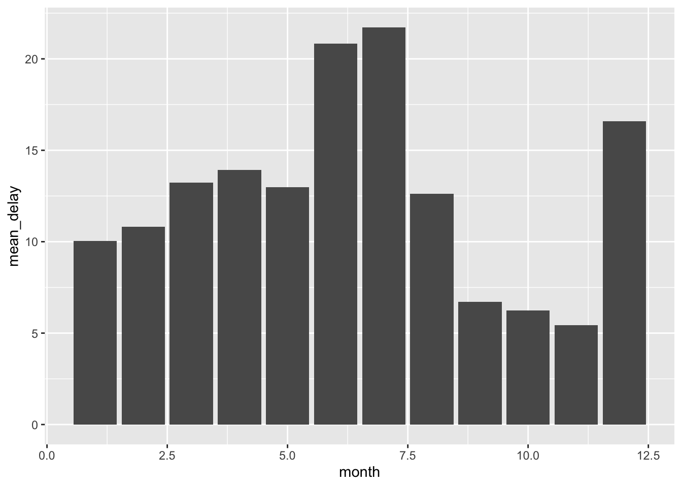
It seems like the most delays happen in the summer and the winter. We can’t be sure with just this data, and we certainly shouldn’t be jumping to any conclusions, but one plausible hypothesis might be that people tend to go on vacation trips during these months, possibly leading to more delays as more flights are in operation.
One useful note to mention is the fact that grouping by multiple variables, then applying a summary effectively peals off one layer of the axis by which the data frame is grouped. This is a mouthful, but let’s see what this means with an example.
per_day <- flights %>%
  group_by(year, month, day) %>%
  summarize(flights = n())

head(per_day)

## # A tibble: 6 x 4
## # Groups:   year, month [1]
##    year month   day flights
##   <int> <int> <int>   <int>
## 1  2013     1     1     842
## 2  2013     1     2     943
## 3  2013     1     3     914
## 4  2013     1     4     915
## 5  2013     1     5     720
## 6  2013     1     6     832
If we apply another summary on this data frame, we obtain
per_month <- per_day %>%
  summarize(flights = sum(flights))

head(per_month)

## # A tibble: 6 x 3
## # Groups:   year [1]
##    year month flights
##   <int> <int>   <int>
## 1  2013     1   27004
## 2  2013     2   24951
## 3  2013     3   28834
## 4  2013     4   28330
## 5  2013     5   28796
## 6  2013     6   28243
Notice that the day column is now gone, and instead we have a data
frame grouped by year and month only. Then, it won’t come as a
surprise that re-applying this step once more would result in
per_year:
per_year <- per_month %>%
  summarize(flights = sum(flights))

head(per_year)

## # A tibble: 1 x 2
##    year flights
##   <int>   <int>
## 1  2013  336776
In this case, the per_year result is uninteresting because the dataset
only pertained to flights that occurred in 2013 to begin with. But if we
had more than one year, then we would expect the results to have shown
up here.
summarize() is not the only function that works well with
group_by(). In fact, we can use it on any function we have learned so
far. For example, here is an example with filter().
flights %>%
  group_by(dest) %>%
  filter(n() > 200)

## # A tibble: 336,053 x 19
## # Groups:   dest [89]
##     year month   day dep_time sched_dep_time dep_delay arr_time
##    <int> <int> <int>    <int>          <int>     <dbl>    <int>
##  1  2013     1     1      517            515         2      830
##  2  2013     1     1      533            529         4      850
##  3  2013     1     1      542            540         2      923
##  4  2013     1     1      544            545        -1     1004
##  5  2013     1     1      554            600        -6      812
##  6  2013     1     1      554            558        -4      740
##  7  2013     1     1      555            600        -5      913
##  8  2013     1     1      557            600        -3      709
##  9  2013     1     1      557            600        -3      838
## 10  2013     1     1      558            600        -2      753
## # … with 336,043 more rows, and 12 more variables: sched_arr_time <int>,
## #   arr_delay <dbl>, carrier <chr>, flight <int>, tailnum <chr>,
## #   origin <chr>, dest <chr>, air_time <dbl>, distance <dbl>, hour <dbl>,
## #   minute <dbl>, time_hour <dttm>
This returns a data frame containing entries for only popular destinations.
Here is another example, this time in combination with filter(),
mutate(), and select().
flights %>%
  filter(arr_delay > 0) %>%
  mutate(prop_delay = arr_delay / sum(arr_delay)) %>%
  select(year: day, dest, arr_delay, prop_delay) %>%
  head()

## # A tibble: 6 x 6
##    year month   day dest  arr_delay prop_delay
##   <int> <int> <int> <chr>     <dbl>      <dbl>
## 1  2013     1     1 IAH          11 0.00000205
## 2  2013     1     1 IAH          20 0.00000373
## 3  2013     1     1 MIA          33 0.00000615
## 4  2013     1     1 ORD          12 0.00000224
## 5  2013     1     1 FLL          19 0.00000354
## 6  2013     1     1 ORD           8 0.00000149
As can be witnessed in these examples, group_by() offers a powerful
way of organizing data, especially when combined with different
operators.
Pipeline Workflow
Let’s take a look at an example from R4DS, which is the task of exploring the relationship between distance and the average delay for each flight destination. Here is one way we might go about it using the pipeline operator and the functions we have learned so far.
dist_delay <- flights %>%
  group_by(dest) %>%
  summarize(
    count = n(),
    mean_dist = mean(distance, na.rm = TRUE),
    mean_delay = mean(arr_delay, na.rm = TRUE)
  ) %>%
  filter(count > 20)

head(dist_delay)

## # A tibble: 6 x 4
##   dest  count mean_dist mean_delay
##   <chr> <int>     <dbl>      <dbl>
## 1 ABQ     254     1826        4.38
## 2 ACK     265      199        4.85
## 3 ALB     439      143       14.4
## 4 ATL   17215      757.      11.3
## 5 AUS    2439     1514.       6.02
## 6 AVL     275      584.       8.00
Now that we have the data ready, let’s try plotting it.
ggplot(data = dist_delay, mapping = aes(x = mean_dist, y = mean_delay)) +
  geom_point(mapping = aes(size = count), alpha = 1/3) +
  geom_smooth(se = FALSE)

## `geom_smooth()` using method = 'loess' and formula 'y ~ x'
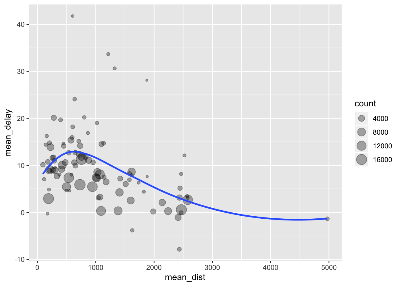
We’ve grouped the data set according to dest, then applied some
summarize function to aggregate the data by mean, then filtered the
results so that we only have destinations that had more than 20 flights
in 2013.Note that we chucked in a function we haven’t seen before,
n(), which basically returns the number of rows in a data frame.
Because we applied a group_by(), the n() would give us the number of
counts of entries for each destination. The ggplot2 aspect of the
workflow should be familiar from the previous tutorial.
We can also use dplyr in conjunction with ggplot2 by using pipe. For
example, say we want to drill down on flight delay times. First, let’s
begin by filtering entries with missing values.
delays <- flights %>%
  filter(!is.na(dep_delay), !is.na(arr_delay)) %>%
  group_by(tailnum) %>%
  summarize(
    count = n(),
    delay = mean(arr_delay)
  )

head(delays)

## # A tibble: 6 x 3
##   tailnum count delay
##   <chr>   <int> <dbl>
## 1 D942DN      4 31.5
## 2 N0EGMQ    352  9.98
## 3 N10156    145 12.7
## 4 N102UW     48  2.94
## 5 N103US     46 -6.93
## 6 N104UW     46  1.80
Using this data frame, we can create a plot as follows:
ggplot(data = delays, mapping = aes(x = count, y = delay)) +
  geom_point(alpha = 1/10)
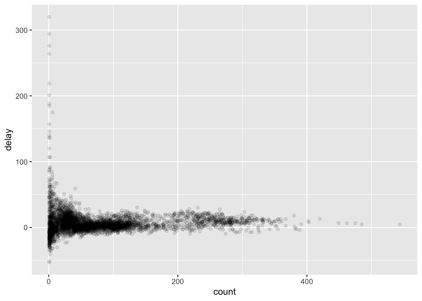
Let’s get rid of some outliers with only a few counts, as they skew the y-axis.
delays %>%
  filter(count > 20) %>%
  ggplot(mapping = aes(x = count, y = delay)) +
    geom_point(alpha = 1/10)
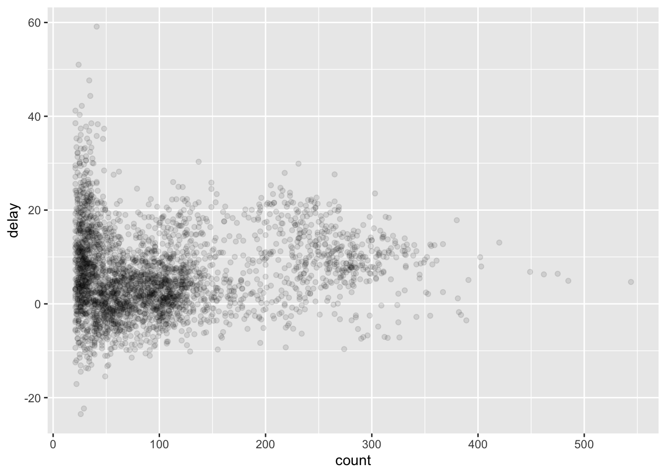
See how we were able to use dpylr data frame manipulation with
ggplot2 directly: we were able to elide the data = delays argument
because the resulting data frame was directly piped into the ggplot()
function.
Conclusion
R4DS Chapter 3 contained a lot of dense information, but the basics of
using pipelines, selecting, mutating, fitering, and group-by’s on data
frames are no doubt useful skills that will come in handy in future
tutorials. I personally don’t think it is necessary to digest everything
that is in the book nor what is written here: instead, it’s important to
see the philosopy of R and dplyr. It’s always fun to learn new syntax
of a language, and I think that’s part of the reason why I’ve enjoyed
writing this post despite the density of the material presented.
I hope you enjoyed reading this post. In the next post, we’ll probably discuss the how-to’s of exploratory data analysis, thus putting our skills to the test. See you in the next one!