VGG PyTorch Implementation
In today’s post, we will be taking a quick look at the VGG model and how to implement one using PyTorch. This is going to be a short post since the VGG architecture itself isn’t too complicated: it’s just a heavily stacked CNN. Nonetheless, I thought it would be an interesting challenge. Full disclosure that I wrote the code after having gone through Aladdin Persson’s wonderful tutorial video. He also has a host of other PyTorch-related vidoes that I found really helpful and informative. Having said that, let’s jump right in.
We first import the necessary torch modules.
import torch
from torch import nn
import torch.nn.functional as F
Let’s first take a look at what the VGG architecture looks like. Shown below is a table from the VGG paper.
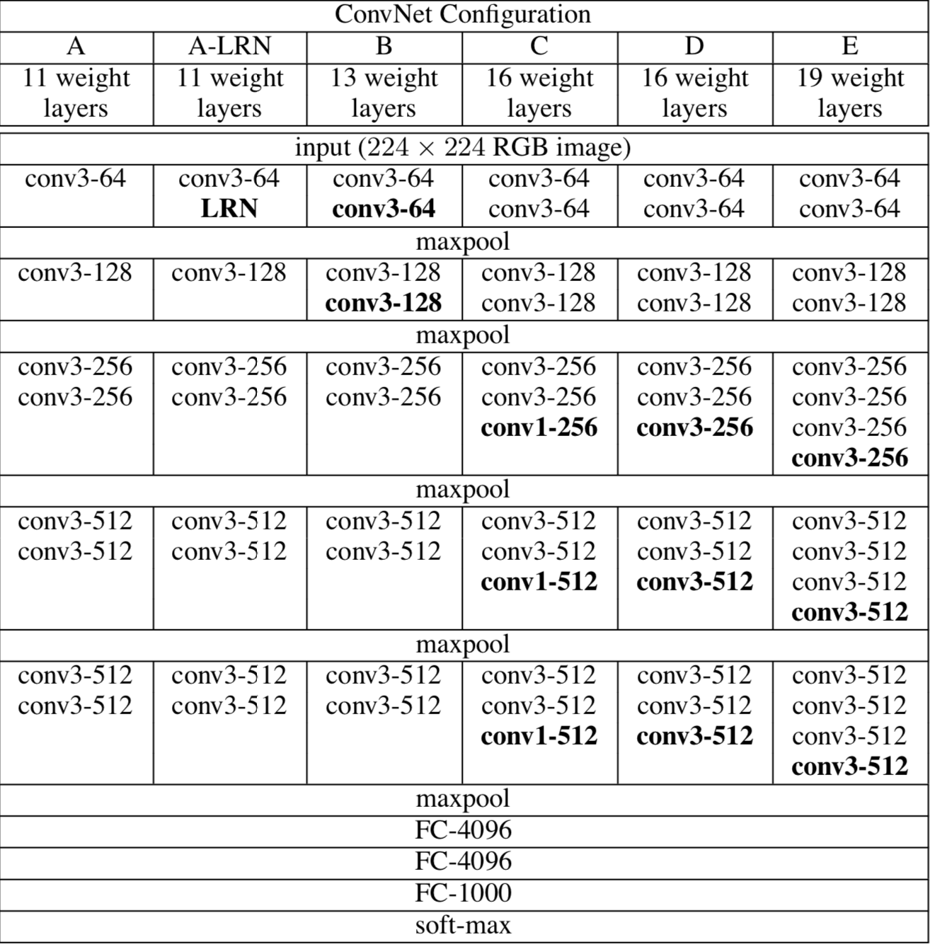
We see that there are a number of different configurations. These configurations typically go by the name of VGG 11, VGG 13, VGG 16, and VGG 19, where the suffix numbers come from the number of layers.
Each value of the dictionary below encodes the architecture information for each model. The integer elements represents the out channel of each layer. "M" represents a max pool layer. You will quickly see that the dictionary is just a simple representation of the tabular information above.
VGG_types = {
    "VGG11": [64, "M", 128, "M", 256, 256, "M", 512, 512, "M", 512, 512, "M"],
    "VGG13": [
        64,
        64,
        "M",
        128,
        128,
        "M",
        256,
        256,
        "M",
        512,
        512,
        "M",
        512,
        512,
        "M",
    ],
    "VGG16": [
        64,
        64,
        "M",
        128,
        128,
        "M",
        256,
        256,
        256,
        "M",
        512,
        512,
        512,
        "M",
        512,
        512,
        512,
        "M",
    ],
    "VGG19": [
        64,
        64,
        "M",
        128,
        128,
        "M",
        256,
        256,
        256,
        256,
        "M",
        512,
        512,
        512,
        512,
        "M",
        512,
        512,
        512,
        512,
        "M",
    ],
}
Now it’s time to build the class that, given some architecture encoding as shown above, can produce a PyTorch model. The basic idea behind this is that we can make use of iteration to loop through each element of the model architecture in list encoding and stack convolutional layers to form a sub-unit of the network. Whenever we encounter "M", we would append a max pool layer to that stack.
class VGG(nn.Module):
    def __init__(
        self,
        architecture,
        in_channels=3,
        in_height=224,
        in_width=224,
        num_hidden=4096,
        num_classes=1000
    ):
        super(VGG, self).__init__()
        self.in_channels = in_channels
        self.in_width = in_width
        self.in_height = in_height
        self.num_hidden = num_hidden
        self.num_classes = num_classes
        self.convs = self.init_convs(architecture)
        self.fcs = self.init_fcs(architecture)

    def forward(self, x):
        x = self.convs(x)
        x = x.reshape(x.size(0), -1)
        x = self.fcs(x)
        return x

    def init_fcs(self, architecture):
        pool_count = architecture.count("M")
        factor = (2 ** pool_count)
        if (self.in_height % factor) + (self.in_width % factor) != 0:
            raise ValueError(
                f"`in_height` and `in_width` must be multiples of {factor}"
            )
        out_height = self.in_height // factor
        out_width = self.in_width // factor
        last_out_channels = next(
            x for x in architecture[::-1] if type(x) == int
        )
        return nn.Sequential(
            nn.Linear(
                last_out_channels * out_height * out_width,
                self.num_hidden),
            nn.ReLU(),
            nn.Dropout(p=0.5),
            nn.Linear(self.num_hidden, self.num_hidden),
            nn.ReLU(),
            nn.Dropout(p=0.5),
            nn.Linear(self.num_hidden, self.num_classes)
        )

    def init_convs(self, architecture):
        layers = []
        in_channels = self.in_channels

        for x in architecture:
            if type(x) == int:
                out_channels = x
                layers.extend(
                    [
                        nn.Conv2d(
                            in_channels=in_channels,
                            out_channels=out_channels,
                            kernel_size=(3, 3),
                            stride=(1, 1),
                            padding=(1, 1),
                        ),
                        nn.BatchNorm2d(out_channels),
                        nn.ReLU(),
                    ]
                )
                in_channels = x
            else:
                layers.append(
                    nn.MaxPool2d(kernel_size=(2, 2), stride=(2, 2))
                )

        return nn.Sequential(*layers)
This is probably the longest code block I’ve written on this blog, but as you can see, the meat of the code lies in two methods, init_fcs() and init_conv(). These methods are where all the fun stacking and appending described above takes place.
I actually added a little bit of customization to make this model a little more broadly applicable. First, I added batch normalization, which wasn’t in the original paper. Batch normalization is known to stabilize training and improve performance; it wasn’t in the original VGG paper because the batch norm technique hadn’t been introduced back when the paper was published. Also, the model above can actually handle rectangular images, not just square ones. Of course, there still is a constraint, which is that the in_width and in_height parameters must be multiples of 32.
BadVGG = VGG(
    in_channels=3,
    in_height=200,
    in_width=150,
    architecture=VGG_types["VGG16"]
)
---------------------------------------------------------------------------

ValueError                                Traceback (most recent call last)

<ipython-input-7-5fd265228616> in <module>
      3     in_height=200,
      4     in_width=150,
----> 5     architecture=VGG_types["VGG16"]
      6 )


<ipython-input-6-78a5ef3a95d1> in __init__(self, architecture, in_channels, in_height, in_width, num_hidden, num_classes)
     16         self.num_classes = num_classes
     17         self.convs = self.init_convs(architecture)
---> 18         self.fcs = self.init_fcs(architecture)
     19
     20     def forward(self, x):


<ipython-input-6-78a5ef3a95d1> in init_fcs(self, architecture)
     29         if (self.in_height % factor) + (self.in_width % factor) != 0:
     30             raise ValueError(
---> 31                 f"`in_height` and `in_width` must be multiples of {factor}"
     32             )
     33         out_height = self.in_height // factor


ValueError: `in_height` and `in_width` must be multiples of 32
Let’s roll out the model architecture by taking a look at VGG19, which is the deepest architecture within the VGG family.
VGG19 = VGG(
    in_channels=3,
    in_height=224,
    in_width=224,
    architecture=VGG_types["VGG19"]
)
If we print the model, we can see the deep structure of convolutions, batch norms, and max pool layers.
print(VGG19)
VGG(
  (convs): Sequential(
    (0): Conv2d(3, 64, kernel_size=(3, 3), stride=(1, 1), padding=(1, 1))
    (1): BatchNorm2d(64, eps=1e-05, momentum=0.1, affine=True, track_running_stats=True)
    (2): ReLU()
    (3): Conv2d(64, 64, kernel_size=(3, 3), stride=(1, 1), padding=(1, 1))
    (4): BatchNorm2d(64, eps=1e-05, momentum=0.1, affine=True, track_running_stats=True)
    (5): ReLU()
    (6): MaxPool2d(kernel_size=(2, 2), stride=(2, 2), padding=0, dilation=1, ceil_mode=False)
    (7): Conv2d(64, 128, kernel_size=(3, 3), stride=(1, 1), padding=(1, 1))
    (8): BatchNorm2d(128, eps=1e-05, momentum=0.1, affine=True, track_running_stats=True)
    (9): ReLU()
    (10): Conv2d(128, 128, kernel_size=(3, 3), stride=(1, 1), padding=(1, 1))
    (11): BatchNorm2d(128, eps=1e-05, momentum=0.1, affine=True, track_running_stats=True)
    (12): ReLU()
    (13): MaxPool2d(kernel_size=(2, 2), stride=(2, 2), padding=0, dilation=1, ceil_mode=False)
    (14): Conv2d(128, 256, kernel_size=(3, 3), stride=(1, 1), padding=(1, 1))
    (15): BatchNorm2d(256, eps=1e-05, momentum=0.1, affine=True, track_running_stats=True)
    (16): ReLU()
    (17): Conv2d(256, 256, kernel_size=(3, 3), stride=(1, 1), padding=(1, 1))
    (18): BatchNorm2d(256, eps=1e-05, momentum=0.1, affine=True, track_running_stats=True)
    (19): ReLU()
    (20): Conv2d(256, 256, kernel_size=(3, 3), stride=(1, 1), padding=(1, 1))
    (21): BatchNorm2d(256, eps=1e-05, momentum=0.1, affine=True, track_running_stats=True)
    (22): ReLU()
    (23): Conv2d(256, 256, kernel_size=(3, 3), stride=(1, 1), padding=(1, 1))
    (24): BatchNorm2d(256, eps=1e-05, momentum=0.1, affine=True, track_running_stats=True)
    (25): ReLU()
    (26): MaxPool2d(kernel_size=(2, 2), stride=(2, 2), padding=0, dilation=1, ceil_mode=False)
    (27): Conv2d(256, 512, kernel_size=(3, 3), stride=(1, 1), padding=(1, 1))
    (28): BatchNorm2d(512, eps=1e-05, momentum=0.1, affine=True, track_running_stats=True)
    (29): ReLU()
    (30): Conv2d(512, 512, kernel_size=(3, 3), stride=(1, 1), padding=(1, 1))
    (31): BatchNorm2d(512, eps=1e-05, momentum=0.1, affine=True, track_running_stats=True)
    (32): ReLU()
    (33): Conv2d(512, 512, kernel_size=(3, 3), stride=(1, 1), padding=(1, 1))
    (34): BatchNorm2d(512, eps=1e-05, momentum=0.1, affine=True, track_running_stats=True)
    (35): ReLU()
    (36): Conv2d(512, 512, kernel_size=(3, 3), stride=(1, 1), padding=(1, 1))
    (37): BatchNorm2d(512, eps=1e-05, momentum=0.1, affine=True, track_running_stats=True)
    (38): ReLU()
    (39): MaxPool2d(kernel_size=(2, 2), stride=(2, 2), padding=0, dilation=1, ceil_mode=False)
    (40): Conv2d(512, 512, kernel_size=(3, 3), stride=(1, 1), padding=(1, 1))
    (41): BatchNorm2d(512, eps=1e-05, momentum=0.1, affine=True, track_running_stats=True)
    (42): ReLU()
    (43): Conv2d(512, 512, kernel_size=(3, 3), stride=(1, 1), padding=(1, 1))
    (44): BatchNorm2d(512, eps=1e-05, momentum=0.1, affine=True, track_running_stats=True)
    (45): ReLU()
    (46): Conv2d(512, 512, kernel_size=(3, 3), stride=(1, 1), padding=(1, 1))
    (47): BatchNorm2d(512, eps=1e-05, momentum=0.1, affine=True, track_running_stats=True)
    (48): ReLU()
    (49): Conv2d(512, 512, kernel_size=(3, 3), stride=(1, 1), padding=(1, 1))
    (50): BatchNorm2d(512, eps=1e-05, momentum=0.1, affine=True, track_running_stats=True)
    (51): ReLU()
    (52): MaxPool2d(kernel_size=(2, 2), stride=(2, 2), padding=0, dilation=1, ceil_mode=False)
  )
  (fcs): Sequential(
    (0): Linear(in_features=25088, out_features=4096, bias=True)
    (1): ReLU()
    (2): Dropout(p=0.5, inplace=False)
    (3): Linear(in_features=4096, out_features=4096, bias=True)
    (4): ReLU()
    (5): Dropout(p=0.5, inplace=False)
    (6): Linear(in_features=4096, out_features=1000, bias=True)
  )
)
We can clearly see the two submodules of the network: the convolutional portion and the fully connected portion.
Now let’s see if all the dimensions and tensor sizes match up. This quick sanity check can be done by passing in a dummy input. This input represents a 3-channel 224-by-224 image.
standard_input = torch.randn((2, 3, 224, 224))
Passing in this dummy input and checking its shape, we can verify that forward propagation works as intended.
VGG19(standard_input).shape
torch.Size([2, 1000])
And indeed, we get a batched output of size (2, 1000), which is expected given that the input was a batch containing two images.
Just for the fun of it, let’s define VGG16 and see if it is capable of processing rectangular images.
VGG16 = VGG(
    in_channels=3,
    in_height=320,
    in_width=160,
    architecture=VGG_types["VGG16"]
)
Again, we can pass in a dummy input. This time, each image is of size (3, 320, 160).
rectangular_input = torch.randn((2, 3, 320, 160))
And we see that the model is able to correctly output what would be a probability distribution after a softmax.
VGG16(rectangular_input).shape
torch.Size([2, 1000])