Neural Style Transfer

In today’s post, we will take a look at neural style transfer, or NMT for short. NMT is something that I first came across about a year ago when reading Francois Chollet’s Deep Learning with Python book. At that time, I was just getting my feet wet in deep learning with Keras, and I specifically remember myself skipping the chapter on NMT, feeling unprepared and intimidated by the implementation. After a full year, I feel ready to face the challenge, but this time with PyTorch. Let’s get started!

Mechanism

Before we get into any specific implementation details, it’s probably helpful to provide some context on how NMT works. Note that, among the many variations of the NMT algorithm, we are going to be discussing the original one first introduced by Gatys et. al.

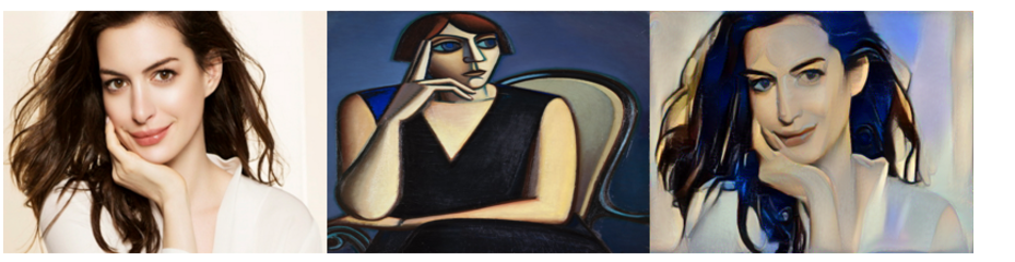
The goal of NMT is simple: given a content image and a style image, transform the content image to have the look and feel of the style image. Below is an example taken from Yunjey’s PyTorch tutorial, which has been an amazing resource so far in my PyTorch journey.

One peculiarity in the original NMT algorithm is that, unlike in typical scenarios in which we update the model’s parameters training, in NMT we update the pixel values of the clone of the content image itself to gradually stylize it. There is no “NMT model” that transforms some image; rather, we merely calculate a loss that is the combination of the content loss and style loss, then optimize the image with respect to this combined loss. Given some style image $S$, content image $C$, and a resulting generated image $G$, we can write the expression for the total loss as

\[L_\text{total}(S, C, G) = L_\text{content} (C, G) + \alpha L_\text{style} (S, G) \tag{1}\]

where $\alpha$ is a weight parameter that determines the degree with which we want to prioritize style over content. Intuitively, the more stylized an image, the higher the content loss; the smaller the content loss, the higher the style loss. In a way, these two quantities are somewhat mutually exclusive, which is why we want to use a weight constant to ascribe some level of importance to one over the other.

Some variations to this formula include those that include weights for both the style and content terms, such as

\[L_\text{total}(S, C, G) = \beta L_\text{content} (C, G) + \alpha L_\text{style} (S, G) \tag{2}\]

At the end of the day, both formulations are identical, only scaled by some scalar value. (2) is a special case of (1) where $\beta = 1$. Thus, we can always go from (1) to (2) simply by multiplying by some constant. For simplicity reasons, we will assume (1) throughout this tutorial.

Content Loss

A natural question to ask, then, is how we calculate each of these loss terms. Somehow, these loss terms should be able to capture how different two images are, content-wise or style-wise. This is where feature extractors come into play.

Pretrained models, such as the VGG network, have filters that are capable of extracting features from an image. It is known that low level convolutional filters that are closer to the input can extract low-level features such as lines or curves, whereas deeper layers are trained to have activation maps that respond to specific shapes or patterns. Notice that this is in line with what the content loss should be able to encode: the general lines and curves of the image should remain similar, as well as the location or presence of general objects like eyes, nose, or hands, to give some concrete examples. Thus, the content loss is simply the L2 norm of the features extracted from each target layer of some pretrained model $m$.

\[L_\text{content}(C, G) = \sum_{l} \sum_{ij} \left( m^l(C)_{ij} - m^l(G)_{ij} \tag{3} \right)^2\]

Do not let the notation confuse you. All this means is that we sum over each layers of the pretrained model $m$. For each of these layers, we calculate matrix element-wise L2 norm of the content and generated image features extracted by the $l$th layer of the model. If we sum all of them up, we obtain the value of the content loss. Intuitively, we can think of this as comparing both high level and low level features between the two images.

Style Loss

The style loss is somewhat trickier, but not too much. The authors of the original NMT paper used what is called the Gram matrix, sometimes also referred to as the Gramian matrix. The Gram matrix, despite its fancy name, is something that you’ve already seen at some point in your study of linear algebra. Given some matrix $A$, the Gram matrix can be calculated as

\[A^\top A\]

More strictly speaking, given a set of vectors $V$, a Gram matrix can be calculated such that

\[G_{ij} = v_i ^\top v_j \tag{4}\]

So how does the Gram matrix encode the stylistic similarities or differences between two images? Before I attempt at an explanation in words, I recommend that you check out this Medium article, which has helped me wrapped my own head around the different dimensions involved in the style loss term. This Medium article has also helped me gain more intuition on why the style loss is the way it is.

The motivating idea is that, given an image and a layer in the feature extractor model, the activations each encode information coming from a filter. The resulting feature maps, therefore, contain information about some feature the model has learned, such as the presence of some pattern, shape, or object. By flattening each feature map and constructing a matrix of activations $A \in \mathbb{R}^{n \times m}$, where $n$ is the number of filters and $m$ is the width times height of each activation, we can now construct the Gram matrix. Effectively, the Gram matrix is a dot product of each rows of $A$; thus, if some $i$th and $j$th features tend to co-occur, $G_{ij}$ will have a large value.

The key here is that the Gram matrix is largely location agnostic; all the information related to locations or positions in the image is lost in the calculation. This is expected, and in some ways desirable, since the style of an image is largely independent from its spatial features. Another key point is that, the style of an image can be thought of as an amalgamation of different combinations of each feature. For instance, Van Gogh’s style of painting is often associated with strong, apparent brush strokes. It is possible to decompose and analyze this style into a set of co-occurring features, such as thick line edges, curves, and so on. So in a sense, the Gram matrix encodes such information at different depths of the pretrained feature extractor, which is why it is fitting to use the Gram matrix for calculating style loss.

Concretely, the equation for style loss goes as follows:

\[L_\text{style}(S, G) = \frac{1}{4 n^2 m^2} \sum_{l} \sum_{ij} (G^l(S)_{ij} - G^l(G)_{ij})^2 \tag{5}\]

The style loss is similar to content loss in the sense that it is also a sum of element-wise L2 norms of two matrices. The differences are that we are using the Gram matrix instead of the raw activations themselves, and that we have a scaling constant. But even this constant is a pretty minor change, as I have seen implementations where the style weight was made a trainable parameter as opposed to a fixed scalar.

Note

As stated earlier, this tutorial seeks to explain the original NMT algorithm. Subsequent NMT methods use an actual model instead of formulating NMT as an optimization problem in which we modify the generated image itself. The benefit of using an actual model is that it is quicker and more efficient; after all, it takes a lot of time to create a plausible image from some white noise (which is why we are going to use the clone of the content image for this tutorial—but even then, it is still very slow).

Now that we have an understanding of how NMT works, let’s get down to the details.

Implementation

Let’s begin by importing necessary modules and handling some configurations for this tutorial.

import os
import torch
from torch import nn
from torchvision import models, transforms
from torchvision.utils import save_image
from PIL import Image
import matplotlib.pyplot as plt
%matplotlib inline
%config InlineBackend.figure_format = 'svg'
device = torch.device('cuda' if torch.cuda.is_available() else 'cpu')

Feature Extractor

We will be using VGG 19 as our pretrained feature extractor model. We will be using five layers of the network to obtain intermediate representations of the input image. Below is a simple code that lets us achieve this task.

class VGG(nn.Module):
    def __init__(self):
        super(VGG, self).__init__()
        self.select = {"0", "5", "10", "19", "28"}
        self.vgg = models.vgg19(pretrained=True).features
    
    def forward(self, x):
        features = []
        for name, layer in self.vgg._modules.items():
            x = layer(x)
            if name in self.select:
                features.append(x)
                if name == "28":
                    break
        return features

In this case, we use the zeroth, fifth, tenth, 19tht, and 28th layers of the model. The output is a list that contains the representations of the input image.

Preprocessing

It’s time to read, load, and preprocess some images. Below is a simple helper function we will use to read an image from some file directory, then apply any necessary resizing and transformations to the image.

def load_image(image_path, shape=None, transform=None):
    image = Image.open(image_path)
    if shape:
        image = image.resize(size, Image.LANCZOS)
    if transform:
        image = transform(image).unsqueeze(0)
    return image.to(device)

Next, let’s define some transformations we will need. The VGG model was trained with a specific transformation configuration, which involves normalizing RGB images according to some mean and standard deviation for each color channel. These values are specified below.

transform = transforms.Compose([
    transforms.ToTensor(),
    transforms.Normalize(
        mean=(0.485, 0.456, 0.406), 
        std=(0.229, 0.224, 0.225)),
])

We will apply this transformation after loading the image. The application of this transformation will be handled by the load_image() function we’ve defined earlier.

Later on in the tutorial, we will also need to undo the transformation to obtain a human presentable image. The following denorm operation accomplishes this task.

denorm = transforms.Normalize(
    (-2.12, -2.04, -1.80), (4.37, 4.46, 4.44)
)

While the numbers might look like they came out of nowhere, it’s actually just a reversal of the operation above. Specifically, given a normalizing operation

\[z = \frac{(x - \mu)}{\sigma}\]

we can undo this normalization via

\[x = \frac{\left(z + \frac{\mu}{\sigma} \right)}{\frac{1}{\sigma}}\]

In other words, the reverse transformation can be summarized as

\[\mu^\prime = - \frac{\mu}{\sigma}, \sigma^\prime = \frac{1}{\sigma}\]

And thus it is not too difficult to derive the values specified in the reverse transformation denorm.

Now, let’s actually load the style and content images. We also create a target image. The original way to create the target image would be to generate some white noise, but I decided to copy the content image instead to make things a little easier and expedite the process. Note also that the code has references to some of my local directories; if you want to test this out yourself, make changes as appropriate.

content = load_image("./data/styles/content.png", transform=transform)
style = load_image(
    "./data/styles/style_3.jpg", 
    transform=transform, 
    shape=[content.size(2), content.size(3)],
)

target_image_path = "./data/styles/generated/output.png"
if os.path.isfile(target_image_path):
    target = load_image(
        target_image_path, transform=transform
    ).requires_grad_(True)
else:
    target = content.clone().requires_grad_(True)

Now we are finally ready to solve the optimization problem!

Optimization

The next step would be to generate intermediate representations of each image, then calculate the appropriate loss quantities. Let’s start by defining some values, such as the learning rate, weights, print steps, and others.

lr = 0.005
style_weight = 120
total_steps = 100
print_step = total_steps // 10
save_step = total_steps // 5
optimizer = torch.optim.Adam([target], lr=lr, betas=[0.5, 0.999])
model = VGG().to(device).eval()

Below is a helper function that we will be using to save images as we optimize. This will help us see the changes in style as we progress throughout the optimization steps.

def generate(target, clamp_val=1, suffix=None):
    img = target.clone().squeeze(0)
    img = denorm(img).clamp_(0, clamp_val)
    if suffix:
        save_path = f"./data/styles/generated/output_{suffix}.png"
    else:
        save_path = f"./data/styles/generated/output.png"
    save_image(img, save_path)

Finally, this is where all the fun part takes place. For each step, we obtain intermediate representations by triggering a forward pass. Then, for each layer, we calculate the content loss and style loss. The code is merely a transcription of the loss equations as defined above. In particular, calculating the Gram matrix might appear a little bit complicated, but all that’s happening is that we are effectively flattening each activation to make it a single matrix, then calculating the Gram via matrix multiplication with its transpose.

for step in range(total_steps):
    target_features = model(target)
    content_features = model(content)
    style_features = model(style)
    
    style_loss = 0
    content_loss = 0
    
    for target_f, content_f, style_f in zip(
        target_features, content_features, style_features
    ):
        content_loss += torch.mean((target_f - content_f) ** 2)
        
        _, c, h, w = content_f.size()
        target_f = target_f.reshape(c, -1)
        style_f = style_f.reshape(c, -1)
        
        target_gram = torch.mm(target_f, target_f.t())
        style_gram = torch.mm(style_f, style_f.t())
        
        style_loss += torch.mean((target_gram - style_gram) ** 2) / (c * h * w) 
    
    loss = content_loss + style_weight * style_loss
    optimizer.zero_grad()
    loss.backward()
    optimizer.step()
    
    if (step + 1) % print_step == 0:
        print(
            f"Step [{step+1}/{total_steps}], "
            f"Content Loss: {content_loss.item():.4f}, "
            f"Style Loss: {style_loss.item():.4f}"
        )
    
    if (step + 1) % save_step == 0:
        generate(target, step + 1)

Step [10/100], Content Loss: 90.1729, Style Loss: 112.5139
Step [20/100], Content Loss: 90.6461, Style Loss: 105.4061
Step [30/100], Content Loss: 92.0474, Style Loss: 100.7770
Step [40/100], Content Loss: 94.7001, Style Loss: 100.8650
Step [50/100], Content Loss: 92.5310, Style Loss: 91.6881
Step [60/100], Content Loss: 93.6766, Style Loss: 88.3200
Step [70/100], Content Loss: 96.4342, Style Loss: 89.8661
Step [80/100], Content Loss: 94.5727, Style Loss: 82.0199
Step [90/100], Content Loss: 93.8605, Style Loss: 82.1147
Step [100/100], Content Loss: 96.4648, Style Loss: 77.7309

We see that style loss decreases quite a bit, whereas the content loss seems to slightly increase with each training step. As stated earlier, it is difficult to optimize on both the content and style, since altering the style of the picture will end up affecting its content in one way or another. However, since our goal is to stylize the target image via NMT, it’s okay to sacrifice a little bit of content while performing NMT, and that’s what is happening here as we can see from the loss values.

Result

And here is the result of the transformation!

save_dir = "./data/styles/generated/custom"
_, axes = plt.subplots(nrows=1, ncols=2)
start_img = Image.open(f"{save_dir}/start.png")
end_img = Image.open(f"{save_dir}/output_200.png")
axes[0].imshow(start_img)
axes[1].imshow(end_img)
_ = [ax.axis("off") for ax in axes]
plt.show()

The result is… interesting, and we certainly see that somethings have changed. We see some more interesting texture in the target image, and there appears to be some changes.

However, at this point, my laptop was already on fire, and more training did not seem to yield any better results. So I decided to try out other sample implementations of NMT to see how using more advanced NMT algorithms could make things any better.

TransformerNet

I decided to try out fast neural style transform, which is available on the official PyTorch GitHub repository. Fast NMT is one of the more advanced, recent algorithms that have been studied after the original NMT algorithm, which we’ve implemente above, was introduced. One of the many benefits of fast neural style transfer is that, instead of framing NMT as an optimization problem, FNMT makes it a modeling problem. In this instance, TransformerNet is a pretrained model that can transform images into their stylized equivalents. The code below was borrowed from the PyTorch repository.

from scripts.style_transfer import TransformerNet

style_model = TransformerNet()
root_dir = "./data/styles/"
state_dict_dir = os.path.join(root_dir, "saved_models")
content_dir = os.path.join(root_dir, "contents")
content_transform = transforms.Compose([
    transforms.ToTensor(),
    transforms.Lambda(lambda x: x.mul(255)),
])
save_dir = os.path.join(root_dir, "generated")

for save_file in os.listdir(state_dict_dir):
    style_name = save_file.split(".")[0]
    state_dict = torch.load(os.path.join(state_dict_dir, save_file))
    state_dict_clone = state_dict.copy()
    for key, _ in state_dict_clone.items():
        if key.endswith(("running_mean", "running_var")):
            del state_dict[key]
    style_model.load_state_dict(state_dict)
    style_model.to(device)
    
    for file_name in os.listdir(content_dir):
        if file_name == ".DS_Store":
            continue
        content_idx = file_name.split(".")[0][-1]
        content = load_image(
            os.path.join(content_dir, file_name), 
            transform=content_transform
        )
        img = style_model(content).detach()[0]
        img = img.clone().clamp(0, 255).numpy()
        img = img.transpose(1, 2, 0).astype("uint8")
        img = Image.fromarray(img)
        file_name = f"output_{style_name}_{content_idx}.png"
        img.save(os.path.join(save_dir, file_name))

I decided to try out FNMT on a number of different pictures of myself, just to see how different results would be for each. Here, we loop through the directory and obtain the file path to each content photo.

generated_files = []

for file_name in os.listdir(save_dir):
    if file_name != ".DS_Store":
        generated_files.append(
            os.path.join(save_dir, file_name)
        )
generated_files.sort()

And here are the results!

nrows = 4
ncols = 5

_, axes = plt.subplots(nrows, ncols, figsize=(12, 12))

for row in range(nrows):
    for col in range(ncols):
        image = Image.open(generated_files[ncols * row + col])
        axes[row, col].imshow(image)
        axes[row, col].axis("off")
plt.show()

Conclusion

Among the 20 photos that have been stylized, I think some definitely look better than others. In particular, I think the third row looks kind of scary, as it made every photo have red hues all over my face. However, there are definitely ones that look good as well. Overall, FNMT using pretrained models definitely yielded better results than our implementation. Of course, this is expected since the original NMT was not the most efficient algorithm; perhaps we will explore FNMT in a future post. But all in all, I think diving into the mechanics behind NMT was an interesting little project.

I hope you’ve enjoyed reading this post. Catch you up in the next one!