My First GAN

Generative models are fascinating. It is no wonder that GANs, or General Adversarial Networks, are considered by many to be where future lies for deep learning and neural networks.

In this post, we will attempt to create a very simple vanilla GAN using TensorFlow. Specifically, our goal will be to train a neural network that is capable of generating compelling images of ships. Although this is a pretty mundane task, it nonetheless sheds lights on the potential that GAN models hold. Let’s jump right into it.

Setup

Below are the dependencies and settings we will be using throughout this tutorial.

import numpy as np
import tensorflow.keras.datasets as tfds
from tensorflow.keras import layers
from tensorflow.keras import optimizers
from tensorflow.keras.models import Model, load_model
from tensorflow.keras.utils import plot_model
from tensorflow.keras.preprocessing import image
%matplotlib inline
%config InlineBackend.figure_format = 'svg'
import matplotlib.pyplot as plt
plt.style.use('seaborn')

Before we start building the GAN model, it is probably a good idea to define some variables that we will be using to configure the parameters of convolutional layers, namely the dimensionality of the images we will be dealing with, as well as the number of color channels and the size of the latent dimension.

latent_dim = 128
height = 32
width = 32
channels = 3

Building the Model

Similar to variational autoencoders, GANs are composed of two parts: the generator and the discriminator. As Ian Goodfellow described in the paper where he first put out the notion of a GAN, generators are best understood as counterfeiters of currency, whereas the discriminator is the police trying to distinguish the fake from the true. In other words, a GAN is a two-component model that involves an internal tug-of-war between two adversarial parties, each trying their best to accomplish their mission. As this competition progresses, the generator becomes increasingly better at creating fake images; the discriminator also starts to excel at determining the veracity of a presented image.

Generator

Enough of theoretical dwellings, let’s begin by defining the generator model. The build_generator is a function that returns a generator model according to some set parameters.

def build_generator(latent_dim, height, width, channels):
  inputs = layers.Input(shape=(latent_dim,))
  x = layers.Dense(128 * 16 * 16)(inputs)
  x = layers.LeakyReLU()(x)
  x = layers.Reshape((16, 16, 128))(x)
  x = layers.Conv2D(256, 5, padding='same')(x)
  x = layers.LeakyReLU()(x)
  x = layers.Conv2DTranspose(256, 4, strides=2, padding='same')(x)
  x = layers.LeakyReLU()(x)
  x = layers.Conv2D(256, 5, padding='same')(x)
  x = layers.LeakyReLU()(x)
  x = layers.Conv2D(256, 5, padding='same')(x)
  x = layers.LeakyReLU()(x)
  output = layers.Conv2D(channels, 7, activation='tanh', padding='same')(x)
  model = Model(inputs, output)
  print(model.summary())
  return model

Let’s take a look at the structure of this network in more detail.

generator = build_generator(latent_dim, height, width, channels)
plot_model(generator, show_shapes=True, show_layer_names=True)

WARNING:tensorflow:From /usr/local/lib/python3.6/dist-packages/tensorflow_core/python/ops/resource_variable_ops.py:1630: calling BaseResourceVariable.__init__ (from tensorflow.python.ops.resource_variable_ops) with constraint is deprecated and will be removed in a future version.
Instructions for updating:
If using Keras pass *_constraint arguments to layers.
Model: "model"
_________________________________________________________________
Layer (type)                 Output Shape              Param #   
=================================================================
input_1 (InputLayer)         [(None, 128)]             0         
_________________________________________________________________
dense (Dense)                (None, 32768)             4227072   
_________________________________________________________________
leaky_re_lu (LeakyReLU)      (None, 32768)             0         
_________________________________________________________________
reshape (Reshape)            (None, 16, 16, 128)       0         
_________________________________________________________________
conv2d (Conv2D)              (None, 16, 16, 256)       819456    
_________________________________________________________________
leaky_re_lu_1 (LeakyReLU)    (None, 16, 16, 256)       0         
_________________________________________________________________
conv2d_transpose (Conv2DTran (None, 32, 32, 256)       1048832   
_________________________________________________________________
leaky_re_lu_2 (LeakyReLU)    (None, 32, 32, 256)       0         
_________________________________________________________________
conv2d_1 (Conv2D)            (None, 32, 32, 256)       1638656   
_________________________________________________________________
leaky_re_lu_3 (LeakyReLU)    (None, 32, 32, 256)       0         
_________________________________________________________________
conv2d_2 (Conv2D)            (None, 32, 32, 256)       1638656   
_________________________________________________________________
leaky_re_lu_4 (LeakyReLU)    (None, 32, 32, 256)       0         
_________________________________________________________________
conv2d_3 (Conv2D)            (None, 32, 32, 3)         37635     
=================================================================
Total params: 9,410,307
Trainable params: 9,410,307
Non-trainable params: 0
_________________________________________________________________
None

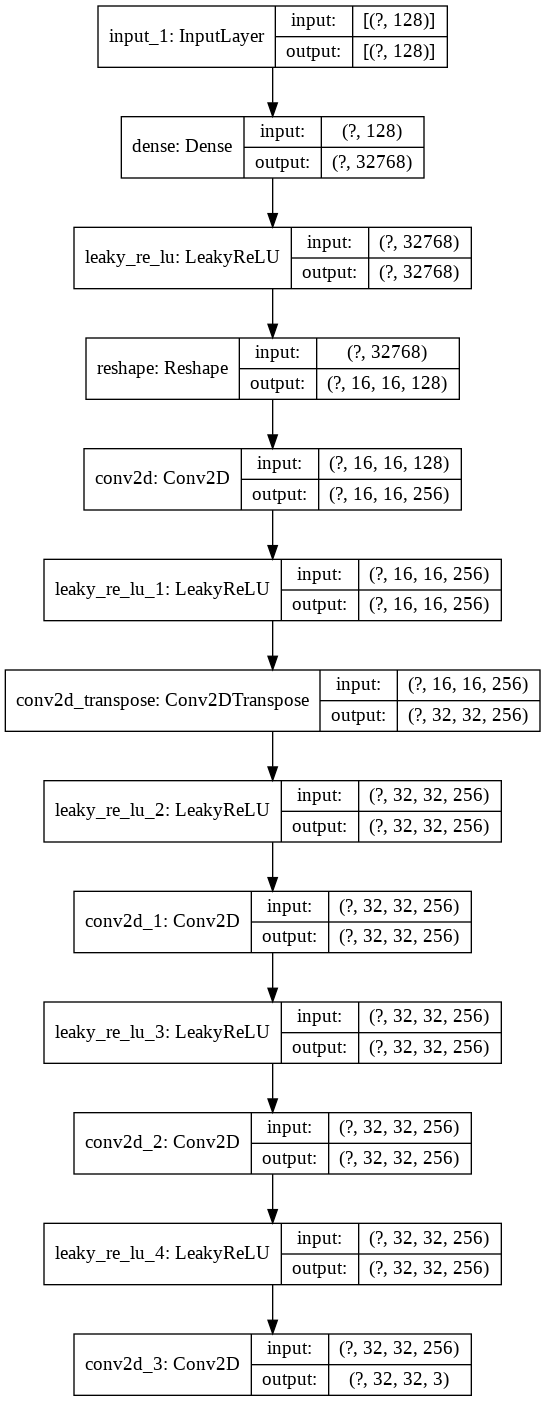
Notice that the output of the generator is a batch image of dimensions (None, 32, 32, 3). This is exactly the same as the height, width, and channel information we defined earlier, and that is no coincidence: in order to fool the discriminator, the generator has to generate images that are of the same dimensions as the training images from ImageNet.

Discriminator

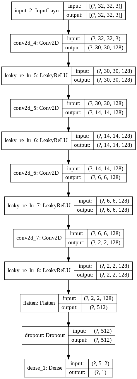
Now it’s time to complete the GAN by creating a corresponding discriminator, the discerning police officer. The discriminator is essentially a simple binary classier that ascertains whether a given image is true or fake. Therefore, it is no surprise that the final output layer will have one neuron with a sigmoid activation function. Let’s take a more detailed look at the build_discriminator function as shown below.

def build_discriminator(height, width, channels):
  inputs = layers.Input(shape=(height, width, channels))
  x = layers.Conv2D(128, 3)(inputs)
  x = layers.LeakyReLU()(x)
  x = layers.Conv2D(128, 4, strides=2)(x)
  x = layers.LeakyReLU()(x)
  x = layers.Conv2D(128, 4, strides=2)(x)
  x = layers.LeakyReLU()(x)
  x = layers.Conv2D(128, 4, strides=2)(x)
  x = layers.LeakyReLU()(x)
  x = layers.Flatten()(x)
  x = layers.Dropout(0.4)(x)
  output = layers.Dense(1, activation='sigmoid')(x)
  model = Model(inputs, output)
  optimizer = optimizers.RMSprop(lr=0.0008, clipvalue=1.0, decay=1e-8)
  model.compile(optimizer=optimizer, loss='binary_crossentropy')
  print(model.summary())
  return model

And again, a model summary for convenient reference:

discriminator = build_discriminator(height, width, channels)
plot_model(discriminator, show_shapes=True, show_layer_names=True)

WARNING:tensorflow:From /usr/local/lib/python3.6/dist-packages/tensorflow_core/python/ops/nn_impl.py:183: where (from tensorflow.python.ops.array_ops) is deprecated and will be removed in a future version.
Instructions for updating:
Use tf.where in 2.0, which has the same broadcast rule as np.where
Model: "model_1"
_________________________________________________________________
Layer (type)                 Output Shape              Param #   
=================================================================
input_2 (InputLayer)         [(None, 32, 32, 3)]       0         
_________________________________________________________________
conv2d_4 (Conv2D)            (None, 30, 30, 128)       3584      
_________________________________________________________________
leaky_re_lu_5 (LeakyReLU)    (None, 30, 30, 128)       0         
_________________________________________________________________
conv2d_5 (Conv2D)            (None, 14, 14, 128)       262272    
_________________________________________________________________
leaky_re_lu_6 (LeakyReLU)    (None, 14, 14, 128)       0         
_________________________________________________________________
conv2d_6 (Conv2D)            (None, 6, 6, 128)         262272    
_________________________________________________________________
leaky_re_lu_7 (LeakyReLU)    (None, 6, 6, 128)         0         
_________________________________________________________________
conv2d_7 (Conv2D)            (None, 2, 2, 128)         262272    
_________________________________________________________________
leaky_re_lu_8 (LeakyReLU)    (None, 2, 2, 128)         0         
_________________________________________________________________
flatten (Flatten)            (None, 512)               0         
_________________________________________________________________
dropout (Dropout)            (None, 512)               0         
_________________________________________________________________
dense_1 (Dense)              (None, 1)                 513       
=================================================================
Total params: 790,913
Trainable params: 790,913
Non-trainable params: 0
_________________________________________________________________
None

Generative Adversarial Network

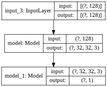
Now we have both the discriminator and the generator, but the two are not really connected in the sense that they exist as discrete models lacking any connection between them. What we want to do, however, is to establish some relationship between the generator and the discriminator to complete a GAN, and hence train them in conjunction. This process of putting the pieces together, or adjoining the models, is where I personally find the genius in GAN design.

The key takeaway here is that we define gan_input and gan_output. As you might imagine, the shape of the input is defined by latent_dim we defined earlier. This is the latent space from which we will sample a random noise vector frame to feed into our GAN. Then, the connection between the generator and the discriminator is effectively established by the statement gan_output = discriminator(generator(gan_input)). All this is saying is that GAN’s output is the evaluation of the generator’s fake image by the discriminator. If the generator does well, it will fool the discriminator and thus output 1; 0 vice versa. Let’s take a look at the code implementation of this logic.

discriminator.trainable = False
gan_input = layers.Input(shape=(latent_dim,))
gan_output = discriminator(generator(gan_input))
gan = Model(gan_input, gan_output)
optimizer = optimizers.RMSprop(lr=0.0004, clipvalue=1.0, decay=1e-8)
gan.compile(optimizer=optimizer, loss='binary_crossentropy')
print(gan.summary())
plot_model(gan, show_shapes=True, show_layer_names=True)

Model: "model_2"
_________________________________________________________________
Layer (type)                 Output Shape              Param #   
=================================================================
input_3 (InputLayer)         [(None, 128)]             0         
_________________________________________________________________
model (Model)                (None, 32, 32, 3)         9410307   
_________________________________________________________________
model_1 (Model)              (None, 1)                 790913    
=================================================================
Total params: 10,201,220
Trainable params: 9,410,307
Non-trainable params: 790,913
_________________________________________________________________
None

Training

Now it’s time to train our model. Let’s first load our dataset. For this, we will be using the cifar10 images. The dataset contains low resolutions images, so our output is also going to be very rough, but it is a good starting point nonetheless.

One hacky thing we do is concatenating the training and testing data. This is because for a GAN, we don’t need to differentiate the two: on the contrary, the more data we have for training, the better. One might suggest that testing data is necessary for the discriminator, which is a valid point, but the end goal here is to build a high performing generator, not the discriminator, so we will gloss over that point for now.

def load_dataset(class_label):
  (X_train, y_train), (X_test, y_test) = tfds.cifar10.load_data()
  X_train = X_train[y_train.flatten() == class_label]
  X_test = X_test[y_test.flatten() == class_label]
  X_train = X_train.astype('float64') / 255.0
  X_test = X_test.astype('float64') / 255.0
  combined_data = np.concatenate([X_train, X_test])
  return combined_data

For this tutorial, we will be using images of ships, which are labeled as 8. So let’s go ahead and specify that.

train_image = load_dataset(8)

We see that train_image contains 6000 images, which is more than enough to start training our GAN.

train_image.shape

(6000, 32, 32, 3)

To train the GAN, we will define a train_gan function. Essentially, this function creates binary labels for real and fake images. Recall that the goal of the discriminator is to successfully discern generated images from real ones. Also recall that to create generated images, the generator needs to sample from a latent dimension. In other words, training will consist of the following steps:

• Sample a random vector to be fed into the generator
• Create zero labels for the corresponding generated images
• Create one labels for real images from the training dataset
• Train the discriminator with the two labels
• Train the GAN by coercing a true label for all images

These high level abstractions are what train_gan implements behind the scenes.

def train_gan(batch_size, iter_num, latent_dim, data, gan_model, generator_model, discriminator_model):
  start = 0
  d_loss_lst, gan_loss_lst = [], []
  for step in range(iter_num):
    random_latent_vectors = np.random.normal(size=(batch_size, latent_dim))
    generated_images = generator_model.predict(random_latent_vectors)
    real_images = data[start: start + batch_size]
    combined_images = np.concatenate([generated_images, real_images])
    labels = np.concatenate([np.zeros((batch_size, 1)),
                             np.ones((batch_size, 1))])
    labels += 0.05 * np.random.random(labels.shape)
    d_loss = discriminator_model.train_on_batch(combined_images, labels)
    d_loss_lst.append(d_loss)

    random_latent_vectors = np.random.normal(size=(batch_size, latent_dim))
    misleading_labels = np.ones((batch_size, 1))
    gan_loss = gan_model.train_on_batch(random_latent_vectors, misleading_labels)
    gan_loss_lst.append(gan_loss)

    if step % 200 == 0:
      print("Iteration {0}/{1}".format(step, iter_num))
      print("[==============================] d-loss: {0:.3f}, gan-loss: {1:.3f}".format(d_loss_lst[-1], gan_loss_lst[-1]))
    
    start += batch_size
    if start > len(data) - batch_size:
      start = 0

  return gan_model, generator_model, discriminator_model, d_loss_lst, gan_loss_lst

There are several subtleties that deserve our attention. First, we fade out the labels ever so slightly to expedite the training process. These are little magic tricks that people have found to work well on GAN training. While I’m not entirely sure about the underlying principle, it most likely comes from the fact that having a smooth manifold is conducive to the training of a neural network.

Second, coercing a true label on the GAN essentially trains the generator. Note that we never explicitly address the generator in the function; instead, we only train the discriminator. By coercing a true label on the GAN, we are effectively forcing the generator to produce more compelling images, and penalizing it when it fails to do so. Personally, I find this part to be the genius and beauty of training GANs.

Now that we have an idea of what the function accomplishes, let’s use it to start training.

batch_size = 32
iter_num = 10000

gan, generator, discriminator, d_history, gan_history = train_gan(batch_size, iter_num, latent_dim, train_image, gan, generator, discriminator)

WARNING:tensorflow:Discrepancy between trainable weights and collected trainable weights, did you set `model.trainable` without calling `model.compile` after ?
Iteration 0/10000
[==============================] d-loss: 0.679, gan-loss: 0.736
Iteration 200/10000
[==============================] d-loss: 0.560, gan-loss: 2.285
Iteration 400/10000
[==============================] d-loss: 0.678, gan-loss: 0.801
Iteration 600/10000
[==============================] d-loss: 0.556, gan-loss: 2.400
Iteration 800/10000
[==============================] d-loss: 0.695, gan-loss: 0.705
Iteration 1000/10000
[==============================] d-loss: 0.699, gan-loss: 0.652
Iteration 1200/10000
[==============================] d-loss: 0.718, gan-loss: 0.606
Iteration 1400/10000
[==============================] d-loss: 0.706, gan-loss: 0.679
Iteration 1600/10000
[==============================] d-loss: 0.675, gan-loss: 0.702
Iteration 1800/10000
[==============================] d-loss: 0.651, gan-loss: 0.668
Iteration 2000/10000
[==============================] d-loss: 0.748, gan-loss: 0.805
Iteration 2200/10000
[==============================] d-loss: 0.682, gan-loss: 0.729
Iteration 2400/10000
[==============================] d-loss: 0.402, gan-loss: 3.102
Iteration 2600/10000
[==============================] d-loss: 0.672, gan-loss: 0.665
Iteration 2800/10000
[==============================] d-loss: 0.659, gan-loss: 0.534
Iteration 3000/10000
[==============================] d-loss: 0.686, gan-loss: 0.679
Iteration 3200/10000
[==============================] d-loss: 0.645, gan-loss: 0.679
Iteration 3400/10000
[==============================] d-loss: 0.681, gan-loss: 0.728
Iteration 3600/10000
[==============================] d-loss: 0.792, gan-loss: 1.180
Iteration 3800/10000
[==============================] d-loss: 0.687, gan-loss: 0.897
Iteration 4000/10000
[==============================] d-loss: 0.791, gan-loss: 1.159
Iteration 4200/10000
[==============================] d-loss: 0.695, gan-loss: 0.680
Iteration 4400/10000
[==============================] d-loss: 0.671, gan-loss: 0.706
Iteration 4600/10000
[==============================] d-loss: 0.702, gan-loss: 0.811
Iteration 4800/10000
[==============================] d-loss: 0.697, gan-loss: 0.634
Iteration 5000/10000
[==============================] d-loss: 0.759, gan-loss: 0.802
Iteration 5200/10000
[==============================] d-loss: 0.677, gan-loss: 0.740
Iteration 5400/10000
[==============================] d-loss: 0.701, gan-loss: 0.663
Iteration 5600/10000
[==============================] d-loss: 0.670, gan-loss: 0.598
Iteration 5800/10000
[==============================] d-loss: 0.615, gan-loss: 0.756
Iteration 6000/10000
[==============================] d-loss: 0.677, gan-loss: 0.626
Iteration 6200/10000
[==============================] d-loss: 0.669, gan-loss: 0.767
Iteration 6400/10000
[==============================] d-loss: 0.682, gan-loss: 0.644
Iteration 6600/10000
[==============================] d-loss: 0.742, gan-loss: 0.955
Iteration 6800/10000
[==============================] d-loss: 0.701, gan-loss: 0.680
Iteration 7000/10000
[==============================] d-loss: 0.303, gan-loss: 7.814
Iteration 7200/10000
[==============================] d-loss: 0.596, gan-loss: 0.847
Iteration 7400/10000
[==============================] d-loss: 0.717, gan-loss: 0.770
Iteration 7600/10000
[==============================] d-loss: 0.707, gan-loss: 0.742
Iteration 7800/10000
[==============================] d-loss: 0.697, gan-loss: 0.795
Iteration 8000/10000
[==============================] d-loss: 0.647, gan-loss: 0.672
Iteration 8200/10000
[==============================] d-loss: 0.676, gan-loss: 0.725
Iteration 8400/10000
[==============================] d-loss: 0.608, gan-loss: 1.050
Iteration 8600/10000
[==============================] d-loss: 0.757, gan-loss: 0.824
Iteration 8800/10000
[==============================] d-loss: 0.614, gan-loss: 0.758
Iteration 9000/10000
[==============================] d-loss: 0.660, gan-loss: 0.647
Iteration 9200/10000
[==============================] d-loss: 0.651, gan-loss: 1.122
Iteration 9400/10000
[==============================] d-loss: 0.710, gan-loss: 0.991
Iteration 9600/10000
[==============================] d-loss: 0.734, gan-loss: 0.901
Iteration 9800/10000
[==============================] d-loss: 0.681, gan-loss: 0.899

The gan-loss seems to fluctuate a bit, which is not necessarily a good sign but also quite a common phenomenon in GAN training. GANs are notoriously difficult to train, since it requires balancing the performance of the generator and the discriminator in such a way that one does not overpower the other. This is referred to as a min-max game in game theory terms, and finding an equilibrium in such structures are known to be difficult.

Result

Let’s take a look at the results now that the iterations are over.

def show_generated_image(generator_model, latent_dim, row_num=4):
  num_image = row_num**2
  random_latent_vectors = np.random.normal(size=(num_image, latent_dim))
  generated_images = generator_model.predict(random_latent_vectors)
  plt.figure(figsize=(10,10))
  for i in range(num_image):
    img = image.array_to_img(generated_images[i] * 255., scale=False)
    plt.subplot(row_num,row_num,i+1)
    plt.grid(False)
    plt.xticks([]); plt.yticks([])
    plt.imshow(img)
  plt.show()

show_generated_image(generator, latent_dim)

The created images are admittedly fuzzy, pixelated, and some even somewhat alien-looking. This point notwithstanding, I find it incredibly fascinating to see that at least some generated images actually resemble ships in the sea. Of particular interest to me are the red ships that appear in [2, 2] and [3, 2]. Given the simplicity of the structure of our network, I would say that this is a successful result.

Let’s take a look at the learning curve of the GAN.

def plot_learning_curve(d_loss_lst, gan_loss_lst):
  fig = plt.figure()
  plt.plot(d_loss_lst, color='skyblue')
  plt.plot(gan_loss_lst, color='gold')
  plt.title('Model Learning Curve')
  plt.xlabel('Epochs'); plt.ylabel('Cross Entropy Loss')
  plt.show()

plot_learning_curve(d_history, gan_history)

As you might expect, the loss is very spiky and erratic. This is why it is hard to determine when to stop training a GAN. Of course, there are obvious signs of failure: when the loss of one component starts to get exponentially larger or smaller than its competitor, for instance. However, this did not happen here, so I let the training continue until the specified number of interactions were over. The results, as shown above, suggest that we haven’t failed in our task.

In a future post, we will be taking a look at the mathematics behind GANs to really understand what’s happening behind the scenes when we pit the generator against its mortal enemy, the discriminator. See you in the next post!