From ELBO to DDPM
In this short post, we will take a look at variational lower bound, also referred to as the evidence lower bound or ELBO for short. While I have referenced ELBO in a previous blog post on VAEs, the proofs and formulations presented in the post seems somewhat overly convoluted in retrospect. One might consider this a gentler, more refined recap on the topic. For the remainder of this post, I will use the terms “variational lower bound” and “ELBO” interchangeably to refer to the same concept. I was heavily inspired by Hugo Larochelle’s excellent lecture on deep belief networks.
Concavity
One important property of the logarithm is that it is a concave function. A function $f$ is concave if it satisfies the following property:
\[f\left( \sum \nolimits_i w_i x_i \right) \geq \sum \nolimits_i f(w_i x_i) \tag{1}\]In other words, if the function evaluated at some weighted sum of values is always greater or equal to the sum of the values evaluated by the function, the function is concave.
As a short detour, we discussed a similar concept in the context of variational autoencoders and Jenson’s inequality in an earlier post. In that post, I introduced the definition of convexity as follows:
\[\mathbb{E}[f(x)] \geq f(\mathbb{E}[x]) \tag{2}\]While the notations used are slightly different, it is easy to see that the this definition is almost the exact reverse of (1). A trivial result of this is that a concave function is convex if and only if it is linear.
Given this understanding, we can now revisit the logarithm and quickly verify that it is a concave function.
Variational Lower Bound
Before diving into a soup of equations, it’s important to remind ourselves of the problem setup. While ELBO is probably most commonly referenced in the context of variational autoencoders, I have recently seen it being mentioned in diffusion models as well. ELBO is a broad concept that can be applied to discuss any model with hidden latent representations, which we will denote as $h$ henceforth.
More concretely, given a model $p(x, h)$, we can write
\[\begin{align} \log p(x) &= \log \left( \sum_{h} p(x, h) \right) \tag{2} \\ &= \log \left( \sum_{h} q(h \vert x) \frac{p(x, h)}{q(h \vert x)} \right) \tag{3} \\ & \geq \sum_{h} q(h \vert x) \log \frac{p(x, h)}{q(h \vert x)} \tag{4} \\ &= \sum_{h} q(h \vert x) \log p(x, h) - \sum_{h} q(h \vert x) \log q(h \vert x) \tag{5} \\ &= \mathbb{E}_q [\log p(x, h) - \log q(h \vert x)] \tag{6} \end{align}\](2) follows from the law of total probability, (3) is a simultaneous application of multiplication and division, (4) follows from the concavity of logarithms, (5) is an algebraic manipulation using the properties of logarithms, and (6) is a rewriting of the expression as an expectation under $q(h \vert x)$.
Equivalence Condition
In the formulation above, $q(h \vert x)$ can be understood as an approximation of a true distribution $p(h \vert x)$. Note that when $q(h \vert x) = p(h \vert x)$, we have an exact equality. Since
\[\log p(x, h) = \log p(h \vert x) + \log p(x)\]We can substitute $q$ for $p$ and rewrite (5) as
\[\begin{align} \log p(x) &= \sum_h p(h \vert x) (\log p(h \vert x) + \log p(x)) - \sum_h p(h \vert x) \log p(h \vert x) \\ &= \sum_h p(h \vert x) \log p(x) \end{align}\]Since $p(x)$ does not depend on $h$, we can pull out the term from the summation, treating it as a constant, leaving us with
\[\log p(x) \sum_h p(h \vert x)\]Using the law of total probability, we see that the summation totals to 1, leaving us with $\log p(x)$, which is what ELBO seeks to approximate.
Variational lower bounds are extremely useful when dealing with models whose interactions between $x$ and the hidden representation $h$ are complex, rendering (2) computationally intractable. Therefore, to train such models, we seek to maximize the log likelihood by pushing the lower bound up.
KL Divergence
Recall the definition of KL divergence:
\[\begin{align} D_\text{KL}(q \parallel p) &= \sum_{x \in X} q(x) \log \left( \frac{q(x)}{p(x)} \right) \\ &= - \sum_{x \in X} q(x) \log \left( \frac{p(x)}{q(x)} \right) \\ \end{align}\]We can see the resemblance between this definition and the definition of ELBO as written in (4), which was
\[\log p(x) \geq \sum_{h} q(h \vert x) \log \frac{p(x, h)}{q(h \vert x)} \tag{4}\]The nice conclusion to this story is that
\[\log p(x) - \text{ELBO} = D_\text{KL}(q(h \vert x) \parallel p(h \vert x)) \tag{7}\]This is a nice interpretation, since KL divergence is by definition always greater or equal to zero. Hence, we can confirm that
\[\log p(x) \geq \text{ELBO}\]Proof
In this section, we sketch a quick proof for (7).
\[\begin{align} D_\text{KL}(q(h \vert x) \parallel p(h \vert x)) &= \mathbb{E}_q [\log q(h \vert x) - \log p(h \vert x) ] \\ &= \mathbb{E}_q [\log q(h \vert x) - \log p(x, h) + \log p(x) ] \\ &= \mathbb{E}_q [\log q(h \vert x) - \log p(x, h)] + \log p(x) \\ \end{align}\]Notice that the expectation is the sign-flipped version ELBO term we derived above.
\[\mathbb{E}_q [\log p(x, h) - q(h \vert x)] \tag{6}\]Therefore, we have
\[D_\text{KL}(q(h \vert x) \parallel p(h \vert x)) = - \text{ELBO} + \log p(x) \\ \implies \log p(x) - \text{ELBO} = D_\text{KL}(q(h \vert x) \parallel p(h \vert x))\]Denoising Diffusion Probabilistic Models
Since we have already seen how ELBO comes up in VAEs, it might be more helpful to take a look at another more recent example I came across while reading Denoising Diffusion Probabilistic Models, or DDPM for short. The intent of this section is not to go over what DDPMs are, but rather to show a sneak peak into how ELBO is mentioned in the paper.
In the paper, the authors write
Training is performed by optimizing the usual variational bound on negative log likelihood: \(\begin{align} \mathbb{E}[- \log p_\theta(\mathbf{x}_0)] & \leq \mathbb{E}_q \left[ - \log \frac{p_\theta (\mathbf{x}_{0:T})}{q(\mathbf{x}_{1:T} \vert \mathbf{x}_0)} \right] \tag{8} \\ &= \mathbb{E}_q \left[ - \log p(\mathbf{x}_T) - \sum_{t \geq 1} \log \frac{p_\theta (\mathbf{x}_{t - 1} \vert \mathbf{x}_t)}{q(\mathbf{x}_t \vert \mathbf{x}_{t - 1})} \right] \tag{9} \\ & := L \end{align}\)
Equation tags have been added for the purposes of this post.
Admittedly, this does look confusing at first sight, but at its core is the definition of ELBO which we have derived in this post, plus some details inherent to DDPMs, such as Markov chain diffusion. In light of the topic of this post, I will attempt to give the simplest possible explanation of the later while focusing on the former.
To make things a little more familiar, let’s rewrite (6) to look more like the one presented in the DDPM paper.
\[\begin{align} \log p(x) & \geq \mathbb{E}_q [\log p(x, h) - \log q(h \vert x)] \tag{6} \\ & \geq \mathbb{E}_q \left[ \log \frac{p(x, h)}{q(h \vert x)} \right] \tag{6-1} \\ \end{align}\]It is not difficult to see that simply flipping sign on both sides results in an expression that closely resembles (8). We also see a one-to-one correspondence between the variables used in this post and the ones in the paper. Namely, $\mathbf{x_0}$ corresponds to $x$, the ground-truth data, and $\mathbf{x}_t$ is the hidden representations of the model.
DDPMs work by starting out with some GT data $\mathbf{x}_0$, then gradually adding Gaussian noise through a Markov chain process. This gradually “breaks” signals originally present in the data, and send the ground truth data to an approximately isotropic distribution. This process is illustrated below. The figure was taken from the author’s website.
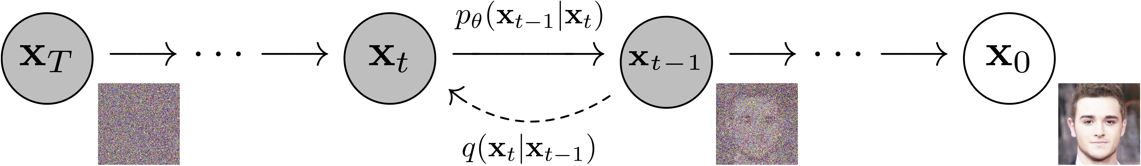
A neural network is then trained to reverse this Markov chain process by recovering the original signal from the noise. The overall intuition is, in some sense, similar to that of GANs or VAEs, where a network learns to map latent dimensions to the data distribution. An obvious difference is that DDPMs iteratively recover the data, whereas GAN generators usually go directly to the data distribution. The slicing and summation notation in (9) exists precisely due to this iterative nature of the DDPM generative process.
Conclusion
Topics like ELBO and KL divergence are one of those concepts that I always think I understand, but do not in reality. The mathematical details underlying those concepts are always intriguing to look at.
While this post in no way covers the entirety of the topic, I hope this will lay a solid foundation for those who want to better understand the mathematics behind latent variable models, such as variational autoencoders, DDPMs and the likes. Personally, I am starting to discover a newfound fascination for DDPMs, and hope to write more about them in the near future.
I hope you enjoyed reading this post. Catch you up in the next one!