On BFS and DFS
In this post, we will be taking a look at a very simple yet popular search algorithm, namely breadth-first search and depth-first search methods. To give you some context, I’ve been solving some simple algorithms problems these days in my free time. I found that thees puzzles are very brain stimulating, not to mention the satisfying sense of reward when my code works. BFS and DFS search methods are widely applicable coding problems, so I decided to write a short post on this topic.
On a separate note, I’m writing this notebook in Jupyter labs instead of Jupyter notebooks. Jupyter labs feels very similar to the former, but the interface is arguably more modern-looking. I’m not sure how I feel Jupyter labs yet, but hopefully as I get to discover more features on this platform, I’ll get a better idea of which interface better suits my workflow.
Let’s get started!
Setup
BFS and DFS are graph search methods. This means that we will need to have a way of representing a graph with code. Of course, the most intuitive way of representing a graph would be to draw it; however, this would be meaningless to a computer. Instead, we will use what is called an adjacency list, which is basically some data structure, mostly a hash map, whose key represents a node and values, the number of connected vertices on the graph. This is one way we can represent information on the vertices and edges of a graph.
graph = {
    'A': ['B'],
    'B': ['A', 'C', 'H'],
    'C': ['B', 'D'],
    'D': ['C', 'E', 'G'],
    'E': ['D', 'F'],
    'F': ['E'],
    'G': ['D'],
    'H': ['B', 'I', 'J', 'M'],
    'I': ['H'],
    'J': ['H', 'K'],
    'K': ['J', 'L'],
    'L': ['K'],
    'M': ['H']
}
This example was borrowed from itholic’s blog. Here is an accompanying image to go along with the hash map.
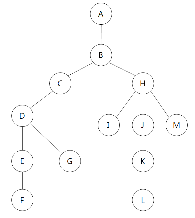
Note that our mode of representation can only express unweighted directed or undirected graphs—that is, the edges between each edges are weightless. To express weighted graphs, we can use something like symmetric matrices, also known as adjacency matrices, that contain information on the distance between each node. Given an adjacency matrix $A$, we would denote the distance between nodes $i$ and $j$ via $A_{ij}$.
Graph representation is an interesting topic, but it is beyond the scope of this post. (We might explore this topic in a future post.) For now, let’s stick with the dictionary representation as shown above and continue probing the world of BFS and DFS.
Breadth First Search
As the name implies, the BFS algorithm is a breadth-based approach. What this means is that we explore each possibility layer by layer: when traversing the graph, we look at the entire picture—hence the breadth—then move onto the next step. Here is a crude analogy for visual thinkers: imagine you have a frappuccino. If BFS were a person, they would drink the first layer—the whipping cream, for instance—then move onto the next. In contrast, Mr. DFS would stick a straw into the cup and drink a little bit of each layer before moving the straw to some other location within the cup and taking a sip again. DFS goes deep, whereas BFS goes wide.
Enough of the coffee analogy, let’s see how we can use BFS to traverse the graph.
def bfs(graph, root):
    visited = set()
    queue = [root]
    while queue:
        node = queue.pop(0)
        if node not in visited:
            visited.add(node)
            queue += graph[node]
    return visited
And here is the result we get when we perform a BFS on the graph. The returned list shows the order in which the nodes in the graph were visited.
bfs(graph, 'A')
['A', 'B', 'C', 'H', 'D', 'I', 'J', 'M', 'E', 'G', 'K', 'F', 'L']
If you look at the visual illustration of the graph above and follow the path that was returned by the bfs() function call, you will quickly see that the order in which the nodes were visited can be understood as level traversal. Recall the Frappuccino analogy, where we said that Mr. BFS would drink the coffee layer-by-layer. The result aligns with our earlier characterization and analogy.
Optimizing with Deques
While there is nothing wrong with the bfs() function as it is, we can perform some slight optimization by using collections.deque (pronounced as “deck”). Notice that in the original bfs() function, we used queue.pop(0) to obtain the first element in the queue. This is a costly operation that takes $O(n)$ time due to the nature of array data structures. The pop() operation itself, which pops the last element of the list, takes only $O(1)$ time complexity, but popping the first element or the head of the list takes linear time.
We can thus use collections.deque’s built-in popleft() to micro-optimize the algorithm.
from collections import deque

def better_bfs(graph, root):
    visited = set()
    queue = deque(root)
    while queue:
        node = queue.popleft()
        if node not in visited:
            visited.add(node)
            queue += graph[node]
    return visited
There is no change in the output path, since the underlying logic remains unchanged.
better_bfs(graph, 'A')
['A', 'B', 'C', 'H', 'D', 'I', 'J', 'M', 'E', 'G', 'K', 'F', 'L']
Depth First Search
Now let’s turn out attention to DFS. As you might be able to tell from the name, DFS first goes deep into the graph until it reaches a leaf node. Then, it traverses the graph back up to its root, then taking another node to deeply search again.
If you look at the dfs() function, you will notice that nothing much has changed from the earlier bfs() function. In fact, the only difference is that we now perform a normal pop() on the list, thus obtaining its last element, instead of doing something like pop(0) or popleft() as we had done above. While this may seem like a very minor difference, the implications of this design choice is substantial: DFS traverses the graph very differently from BFS.
def dfs(graph, root):
    visited = set()
    stack = [root]
    while stack:
        node = stack.pop()
        if node not in visited:
            visited.add(node)
            stack += graph[node]
    return visited
The key difference is that DFS goes down the graph, then comes back up, repeating this up-and-down motion until all nodes are visited. This vertical movement can also be understood, from a level’s perspective, as depth—hence the name, DFS.
dfs(graph, 'A')
['A', 'B', 'H', 'M', 'J', 'K', 'L', 'I', 'C', 'D', 'G', 'E', 'F']
Recursion
The implementation of the DFS traversing algorithm above used iteration with a while loop. However, we can also use recursion with an inner helper function to populate the results list, then return the populated result. This uses the convenient fact that we can have nested functions in Python with an internal local variable whose scope is effectively global for the inner function.
def dfs_recursive(graph, node):
    visited = set()
    def _helper(node):
        if node not in visited:
            visited.add(node)
            for child in graph[node][::-1]:
                _helper(child)
    _helper(node)
    return visited
If you think about the order in which the recursive calls are being made in the function, it will become obvious that the stack we had in the iterative version of the DFS algorithm was basically simulating an actual stack frame on the computer with recursion. In other words, the two methods achieve the same functionality, albeit in seemingly different ways.
dfs_recursive(graph, 'A')
['A', 'B', 'H', 'M', 'J', 'K', 'L', 'I', 'C', 'D', 'G', 'E', 'F']
Path Finding
An interesting application of the DFS and BFS algorithms is in the context of path finding. In the examples above, we simply traversed the entire graph in order determined by the algorithm, given a starting node. However, what if we want to find ways to get from node X to node Y? The traversing algorithm does not answer this question directly. So let’s use these algorithms to answer the question in a more direct manner.
Note that finding the longest or shortest path from one node to another is considered an NP-hard problem, which means that it is a very difficult problem to which computer scientists and mathematicians have yet to find an answer for. The DFS or BFS approach outlined below is a very crude way of going about this problem and can hardly be called as a solution given the exponential amount of computation that is needed to perform on much complicated graphs. With this bearing in mind, let’s take a look.
DFS Approach
In the example below, we use DFS to find one possible path from start to end. Note that this may not be the quickest path, since DFS is unable to look at the graph level by level—for that, we will need BFS.
def dfs_path(graph, start, end):
    visited = set()
    stack = [[start]]
    while stack:
        path = stack.pop()
        for node in graph[path[-1]]:
            if node not in visited:
                visited.add(node)
                temp = path.copy()
                temp.append(node)
                if node == end:
                    return temp
                else:
                    stack.append(temp)
Check that the function works as expected.
dfs_path(graph, 'A', 'L')
['A', 'B', 'H', 'J', 'K', 'L']
BFS Approach
Next, here is the same path finding algorithm using BFS. The code is nearly identical to the DFS model we’ve seen above, but because this algorithm uses level order traversal, we can say with more confidence that the returned result is the shortest path from start to end. We also apply the micro-optimization method we reviewed earlier with collections.deque().
def bfs_path(graph, start, end):
    visited = set()
    queue = deque([[start]])
    while queue:
        path = queue.popleft()
        for node in graph[path[-1]]:
            if node not in visited:
                visited.add(node)
                temp = path.copy()
                temp.append(node)
                if node == end:
                    return temp
                else:
                    queue.append(temp)
Because we had a very simple example, it turns out that the method we found with DFS was in fact the shortest path.
bfs_path(graph, 'A', 'L')
['A', 'B', 'H', 'J', 'K', 'L']
Searching All Paths
The methods above return an efficient path from start to end. But what if we want to know all possible paths that are possible, even if some of them might be elongated or inefficient?
The idea is that we specify a set number of iterations we want the algorithm to run for, denoted in the function parameter as n_iter. During that n_iter, we find all paths that are possible. When the iterations are over, we return the result.
def find_all_paths(graph, start, end, n_iter):
    paths = []
    queue = deque([[start]])
    for _ in range(n_iter):
        path = queue.popleft()
        for node in graph[path[-1]]:
            temp = path.copy()
            temp.append(node)
            if node == end:
                paths.append(temp)
            else:
                queue.append(temp)
    return paths
Let’s try running this for a hundred iterations and see what we get.
find_all_paths(graph, 'A', 'L', 100)
[['A', 'B', 'H', 'J', 'K', 'L'],
 ['A', 'B', 'A', 'B', 'H', 'J', 'K', 'L'],
 ['A', 'B', 'C', 'B', 'H', 'J', 'K', 'L']]
Great! Note that the path we get all starts with 'A' and ends with 'L', which is what we had specified. One problem, however, is the fact that besides the first path, the second and third paths include somewhat ineffective paths, where the walker presumably goes from 'A' to 'B', then back to 'A', and so on. This problem becomes even more apparent when we run it for more iterations.
find_all_paths(graph, 'A', 'L', 500)
[['A', 'B', 'H', 'J', 'K', 'L'],
 ['A', 'B', 'A', 'B', 'H', 'J', 'K', 'L'],
 ['A', 'B', 'C', 'B', 'H', 'J', 'K', 'L'],
 ['A', 'B', 'H', 'B', 'H', 'J', 'K', 'L'],
 ['A', 'B', 'H', 'I', 'H', 'J', 'K', 'L'],
 ['A', 'B', 'H', 'J', 'H', 'J', 'K', 'L'],
 ['A', 'B', 'H', 'J', 'K', 'J', 'K', 'L'],
 ['A', 'B', 'H', 'M', 'H', 'J', 'K', 'L'],
 ['A', 'B', 'A', 'B', 'A', 'B', 'H', 'J', 'K', 'L'],
 ['A', 'B', 'A', 'B', 'C', 'B', 'H', 'J', 'K', 'L'],
 ['A', 'B', 'A', 'B', 'H', 'B', 'H', 'J', 'K', 'L'],
 ['A', 'B', 'A', 'B', 'H', 'I', 'H', 'J', 'K', 'L'],
 ['A', 'B', 'A', 'B', 'H', 'J', 'H', 'J', 'K', 'L'],
 ['A', 'B', 'A', 'B', 'H', 'J', 'K', 'J', 'K', 'L'],
 ['A', 'B', 'A', 'B', 'H', 'M', 'H', 'J', 'K', 'L'],
 ['A', 'B', 'C', 'B', 'A', 'B', 'H', 'J', 'K', 'L'],
 ['A', 'B', 'C', 'B', 'C', 'B', 'H', 'J', 'K', 'L']]
Non-overlapping Paths
If we want to obtain only those results that are non-overlapping, we can add a manual check, i.e. add only those results that have unique nodes. We add this check by adding a control statement, namely if node not in path:. This ensures that the node that we are considering is not a node that the path had already visited before.
def find_non_overlapping_paths(graph, start, end, n_iter):
    paths = []
    queue = deque([[start]])
    for _ in range(n_iter):
        if not queue:
            break
        path = queue.popleft()
        for node in graph[path[-1]]:
            if node not in path:
                temp = path.copy()
                temp.append(node)
                if node == end:
                    paths.append(temp)
                else:
                    queue.append(temp)
    return paths
And if we run this on the graph, we obtain the result that we had expected.
find_non_overlapping_paths(graph, 'A', 'L', 100)
[['A', 'B', 'H', 'J', 'K', 'L']]
However, this is a rather boring example. Let’s alter the graph a bit by adding a bidirectional connection between nodes 'G'and 'I'. Notice that this creates an internal loop within the graph. In graph theory language, this is known as a strongly connected component, and we might explore this topic in a future post. For now, we can understand them as a loop, the implication of which is that there are now multiple ways to get from one node to another via that loop.
graph2 = graph.copy()
graph2['G'] = ['D', 'I']
graph2['I'] = ['H', 'G']
This time, when we run the path finding algorithm, we find (no pun intended) that there are two ways of going from node 'A' to node 'I'.
find_non_overlapping_paths(graph2, 'A', 'I', 100)
[['A', 'B', 'H', 'I'], ['A', 'B', 'C', 'D', 'G', 'I']]
Example Problems
In this last section, we will take a look at two LeetCode BFS-related problems.
One thing that I have slowly realized is that, solving a coding puzzle does not mean that I have understood the problem. In fact, more often or not, I’ve found myself struggling to solve problems that I somehow managed to solve weeks or months ago. I’ve therefore decided that it is good practice to come back to previous problems once in a while for review.
Binary Tree Level Traversal
The first problem is Problem 102. This involves level-order traversal of a binary search tree. Upon reading this question, a small voice in you should be yelling “BFS, BFS!”, because we have repeated many times that BFS is reminiscent of level-order traversal, where we search a tree or a graph layer by layer.
Here is my solution.
class TreeNode:
    def __init__(self, val=0, left=None, right=None):
        self.val = val
        self.left = left
        self.right = right


def levelOrder(root: TreeNode):
    visited = []
    if not root:
        return visited
    to_visit = [root]
    while to_visit:
        values = []
        next_nodes = []
        for node in to_visit:
            if node:
                values.append(node.val)
                next_nodes += [node.left, node.right]
        if values:
            visited.append(values)
        to_visit = next_nodes
    return visited
The idea is pretty simple: in to_visit, we keep track of nodes to visit. These nodes obviously live in the same level. Then, we loop through this list of nodes. If the node is not None, we add its value to a temporary list within the while loop, denoted as values. When we are done traversing the nodes in that level, we append the accumulated results of value to visited. We also keep track of the next layer via next_nodes. This next_nodes contains the nodes to visit in the next iteration, so it becomes the new to_visit. In the next iteration, we repeat what we have done on the next_nodes list until there is no more nodes to traverse, i.e. we are at the leaf nodes.
Symmetric Binary Tree
This is Problem 101 on LeetCode. The problem is simple: we want to check if a binary tree is symmetric. An example of a symmetric tree is visualized below:
    1
   / \
  2   2
 / \ / \
3  4 4  3
How might we go about this? My initial thought was that we could use level order traversal and check if, at each level, the values of the node are symmetric. This check of symmetry can be done simply by doing something like a palindrome check, i.e. values == values[::-1]. However, upon more research and thinking, I’ve realized that there are smarter ways to do this by using queues.
def isSymmetric(root: TreeNode) -> bool:
    if not root:
        return True
    queue = collections.deque([[root.left, root.right]])
    while queue:
        left, right = queue.popleft()
        if left == right == None:
            continue
        if left and right is None or right and left is None:
            return False
        if left.val != right.val:
            return False
        queue += [[left.left, right.right], [left.right, right.left]]
    return True
All we have to do is to make sure that the value of the left and right nodes are identical. If they are, now we need to check if the value of the left child of the left node is equal to that of the right child of the right node. This is the outer-layer comparison, represented as [left.left, right.right]. For an inner layer comparison, we need to check if the value of the right child of the left node is equal to that of the left child of the right node. This corresponds to [left.right, right.left]. In the example above, for instance, we need to check that 4 and 4 are equal, and also that 3 and 3 are equal in the outer most leaf nodes. We add these to the queue so that comparisons can be made in the iterations that follow.
Conclusion
In this post, we looked at BFS and DFS algorithms. These algorithms are very useful for traversing a tree structure. A generalization of DFS, for example, is the backtracking algorithm, which is often used to solve many problems. Although there is nothing special about DFS and BFS in that they are essentially brute force methods of search, they are nonetheless powerful tools that can be used to tackle countless tasks. It’s also just good exercise with Python.
I hope you’ve enjoyed reading this blog. Catch you up in the next one.