Better seq2seq

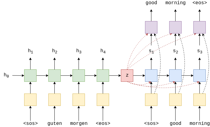
In the previous post, we took a look at how to implement a basic sequence-to-sequence model in PyTorch. Today, we will be implementing a small improvement to the previous model. These improvements were suggested in Learning Phrase Representations using RNN Encoder-Decoder for Statistical Machine Translation, by Cho, et. al. To cut to the chase, the image below, taken from Ben Trevett’s tutorial, encapsulates the enhancement we will be implementing today.

In the previous model, the hidden state of the model was a bottleneck: all the information from the encoder was supposed to be compressed into the hidden state, and even that encoder hidden state would have undergone changes as the decoder was unrolled with subsequent target sequences.

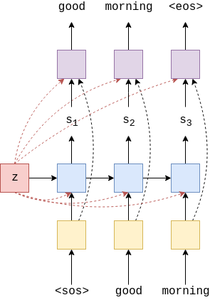
To reduce this bottleneck and lessen the compression burden on the encoder hidden state, the improved architecture will allow the decoder to gain access to the encoder hidden state at each time step. Moreover, the final classifier output layer in decoder will have access to the original embedding of the target language token as well as the last hidden state of the encoder, represented as $z$ in the diagram above. This can be considered a residual connection, since the embedding skips the RNN and directly gets fed into the fully connected layer.

Now that we have some idea of what we want to achieve, let’s start coding.

Implementation

Since the setup for this tutorial is identical to that of the previous post, I’ll skip much of the explanation and sanity checks. In the code block below, we load the Multi30k dataset, then create bucket iterators for each train, validation, and test split.

import random
import time

import torch
import torchtext
from torch import nn
from torchtext.data import BucketIterator, Field
from torchtext.datasets import Multi30k


SRC = Field(
    tokenize="spacy",
    tokenizer_language="de",
    init_token="<sos>",
    eos_token="<eos>",
    lower=True,
)

TRG = Field(
    tokenize="spacy",
    tokenizer_language="en",
    init_token="<sos>",
    eos_token="<eos>",
    lower=True,
)

train_data, validation_data, test_data = Multi30k.splits(
    root="data", exts=(".de", ".en"), fields=(SRC, TRG)
)

SRC.build_vocab(train_data, max_size=10000, min_freq=2)
TRG.build_vocab(train_data, max_size=10000, min_freq=2)

BATCH_SIZE = 128
device = torch.device('cuda' if torch.cuda.is_available() else 'cpu')

train_iterator, validation_iterator, test_iterator = BucketIterator.splits(
    (train_data, validation_data, test_data), batch_size=BATCH_SIZE, device=device
)

Encoder

Let’s start with the encoder. The encoder here is actually almost identical to the one we implemented in the previous model. In fact, it is arguably simpler, as we are now using a single GRU layer instead of a two-layered LSTM.

class Encoder(nn.Module):
    def __init__(self, vocab_size, embed_dim, hidden_size, dropout):
        super(Encoder, self).__init__()
        self.dropout = nn.Dropout(dropout)
        self.embed = nn.Embedding(vocab_size, embed_dim)
        self.gru = nn.GRU(embed_dim, hidden_size)

    def forward(self, x):
        embedding = self.dropout(self.embed(x))
        outputs, hidden = self.gru(embedding)
        return hidden

Decoder

The decoder is where all the enhancements are going to take place. Recall the changes we want to make to the previous seq2seq architecture.

As you can see, we need to make sure that

• the encoder hidden states are accessible at all time steps
• the encoder hidde states and embeddings should be passed to the fully connected classifier

The first change means that the decoder’s forward method needs to be able to take in the encoder’s hidden states as input. For sake of notational clarity, let’s call those hidden states as “context.” The way we allow the decoder to use its own hidden state as well as the context for computation is that we concatenate the context with its input embeddings. Effectively, we could think of this as creating a new embedding vectors, where the first half comes from actual embeddings of English tokens and the later half comes from the context vector.

class Decoder(nn.Module):
    def __init__(self, vocab_size, embed_dim, hidden_size, dropout):
        super(Decoder, self).__init__()
        self.vocab_size = vocab_size
        self.dropout = nn.Dropout(dropout)
        self.embed = nn.Embedding(vocab_size, embed_dim)
        self.gru = nn.GRU(embed_dim + hidden_size, hidden_size)
        self.fc = nn.Linear(embed_dim + hidden_size * 2, vocab_size)
        
    def forward(self, x, hidden, context):
        # x.shape == (128,)
        # context.shape == (1, 128, 512)
        x = x.unsqueeze(0)
        # x.shape == (1, 128)
        embedding = self.dropout(self.embed(x))
        # embedding.shape == (1, 128, 256)
        embed_context = torch.concat((embedding, context), dim=2)
        # embed_context.shape == (1, 128, 768)
        _, hidden = self.gru(embed_context, hidden)
        # hidden.shape = (1, 128, 512)
        outputs = torch.cat(
            (embedding.squeeze(0), hidden.squeeze(0), context.squeeze(0)), 
            dim=1)
        predictions = self.fc(outputs)
        return predictions, hidden

Another implementation detail not mentioned earlier is the dimension of the last fully connected classifier layer. Since we now concatenate the embedding vector with the hidden state from the GRU, context vector from the encoding, as well as the original embedding vectors, the classifier’s input dimensions are much larger than they were in the previous decoder model.

Seq2seq

Now it’s time to implement the sequence-to-sequence model. Most of the enhancements were already baked into the decoder, and the fundamental logic through which predictions are generated remain unchanged. Thus, only minimal changes have to be made to the seq2seq model: namely, we need to handle the context vector and pass it to the decoder at every time step.

class Seq2Seq(nn.Module):
    def __init__(self, encoder, decoder, device):
        super(Seq2Seq, self).__init__()
        self.encoder = encoder
        self.decoder = decoder
        self.device = device
    
    def forward(self, source, target, teacher_force_ratio=0.5):
        seq_len = target.size(0)
        batch_size = target.size(1)    
        outputs = torch.zeros(
            seq_len, batch_size, self.decoder.vocab_size
        ).to(self.device)
        
        context = self.encoder(source)
        hidden = context
        x = target[0]
        
        for t in range(1, seq_len):
            predictions, hidden = self.decoder(x, hidden, context)
            outputs[t] = predictions
            teacher_force = random.random() < teacher_force_ratio
            if teacher_force:
                x = predictions.argmax(1)
            else:
                x = target[t]
                
        return outputs

And from here on, the details are exactly identical; the same train() and evaluate() functions can be used in the previous post. Since I intended this post to be a simple little exercise as opposed to a fully blown out tutorial, we’ll stop here, but by all means, feel free to experiment more with it. Below are the configurations Ben Trevett used in his tutorial.

INPUT_DIM = len(SRC.vocab)
OUTPUT_DIM = len(TRG.vocab)
ENC_EMB_DIM = 256
DEC_EMB_DIM = 256
HID_DIM = 512
ENC_DROPOUT = 0.5
DEC_DROPOUT = 0.5

encoder = Encoder(INPUT_DIM, ENC_EMB_DIM, HID_DIM, ENC_DROPOUT)
decoder = Decoder(OUTPUT_DIM, DEC_EMB_DIM, HID_DIM, DEC_DROPOUT)
model = Seq2Seq(encoder, decoder, device).to(device)

When I was writing this notebook, I realized that I enjoy thinking about the dimensional details of each tensor being passed around here and there. It is difficult, and sometimes it required me to use dirty print statements to actually log what was happening to each variable, but all in all, I think attention to dimensional detail is definitely something that one should practice and think about when modeling.

I hope you enjoyed reading this post. In a future post, we will explore what attention is and how to bake it into a seq2seq model to take it to the next level.

Also, happy holidays!